Growing or Compressing Datasets
For supervised learning applications where training data have been annotated by humans, labeling is time-consuming and expensive. This lecture focuses on ways to more carefully select what examples to label and reduce the labeling burden of creating modern ML systems. Specifically, we look at the following approaches:
- Active learning as a way to intelligently select examples to label and grow datasets
- Core-set selection to compress datasets down to a representative subset.
We will focus on classification tasks, but these ideas apply to other supervised learning tasks (regression, image segmentation, entity recognition, etc.) and some unsupervised learning tasks (e.g., summarization).
Active learning
The goal of active learning is to select the best examples to label next in order to improve our model the most. Suppose our examples have feature values $x$ which are inputs to model $A$ that is trained to output accurate predictions $A(x)$. For instance in image classification applications, we might have: examples which are images, feature values which are pixel intensities, a model that is some neural network classifier, and model outputs which are predicted class probabilities.
Often we can use these outputs from an already-trained model to adaptively decide what additional data should be labeled and added to the training dataset, such that retraining this model on the expanded dataset will lead to greatest boost in model accuracy. Using active learning, you can train a model with much fewer labeled data and still achieve the same accuracy as a model trained on a much larger dataset where what data to label was selected randomly.
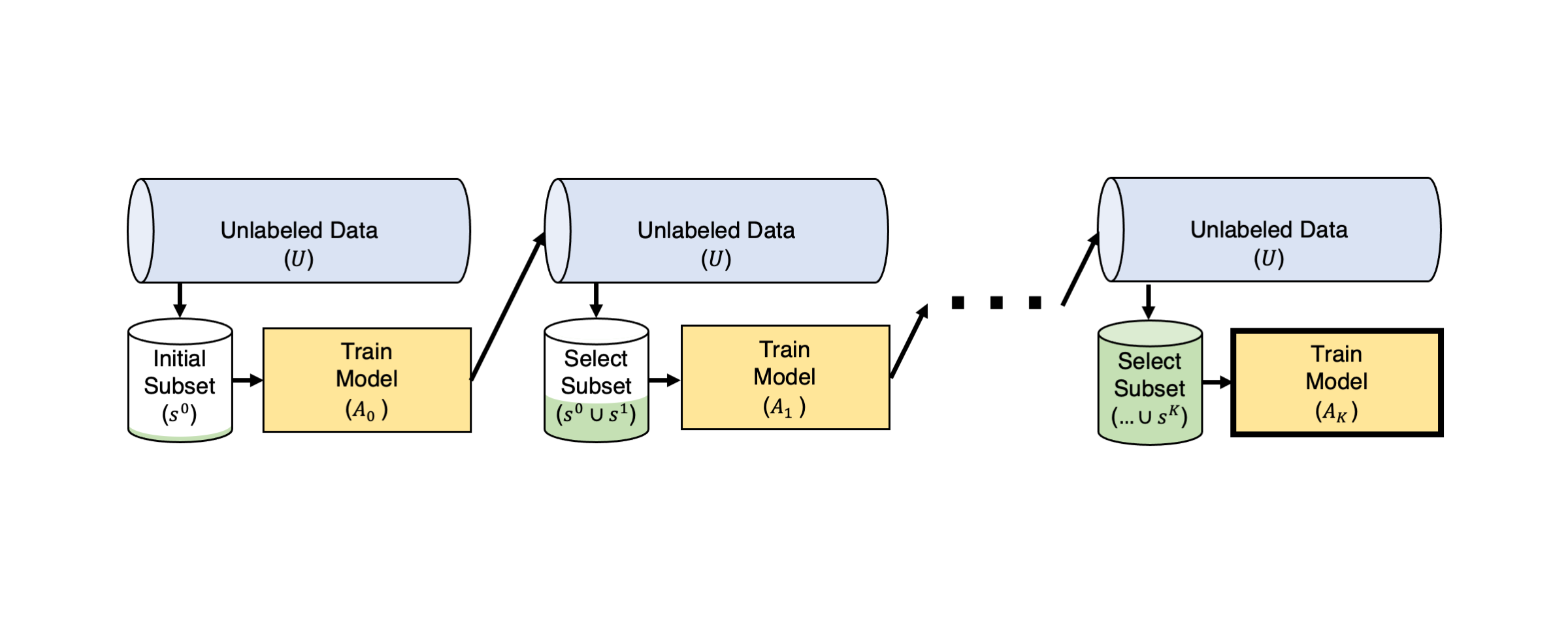
In pool-based active learning, there exists a pool of currently unlabeled examples $U$. We label this data iteratively in multiple rounds $r = 1,2, …, T$. Each round involves the following steps:
- Compute outputs from our model trained on the currently-labeled data from the previous round $A_r$ (for example obtaining probabilistic predictions for each unlabaled example).
- Use these model outputs together with an active learning algorithm $\phi$ that scores each unlabeled example $x \in U$ in order to determine which data would be most informative to label next. Here the acquisition function $\phi(x, A_r)$ estimates the potential value of labeling a particular datapoint (i.e. how much is adding this datapoint to our current training set expected to improve the model), based on its feature value and the output of the trained model from the previous round $A_r(x)$.
- Actually collect the labels for the data suggested by our active learning algorithm and add these labels examples to our training data for the next round: $D_{r+1}$ (removing these examples from $U$ once they are labeled).
- Train our model on the expanded dataset $D_{r+1}$ to get a new model $M_{r+1}$.
In classification tasks with $K$ classes, the model outputs a vector of predicted class probabilities $ \mathbf{p} = [p_1, p_2, …, p_K] = A_r(x)$ for each example $x$. Here a common acquisition function is the entropy of these predictions as a form of uncertainty sampling:
\[\phi(x, A_r) = - \sum_{k} p_k \log p_k\]This $\phi(x, A_r)$ takes the largest values for those unlabeled examples that our current model has the most uncertainty about. Labeling these examples is potentially much more informative than others since our model is currently very unsure what to predict for them.
The active learning process is typically carried out until a labeling budget is reached, or until the model has achieved desired level of accuracy (evaluated on a separate held-out validation set).
Passive vs Active Learning
Here we present a simple 1-dimensional example that illustrates the value of active learning. We compare against a “passive learning” algorithm that randomly selects which data to label next in each round.
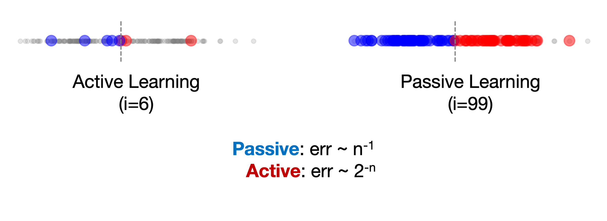
In this simple 1-D example, active learning quickly selects samples to hone in on the actual decision boundary (represented by the dashed gray line), effectively performing a binary search to reach the boundary in about 6 iterations. On the other hand, passive learning (or random sampling) takes much longer because it relies on randomness to get examples close to the decision boundary, taking close to 100 iterations to reach a similar point as the active approach! Theoretically, active learning can exponentially speed up data efficiency compared to passive learning, in terms of the amount of data $n$ needed to reach a goal model error rate ($2^{-n}$ for active vs. $n^{-1}$ for passive in this case).
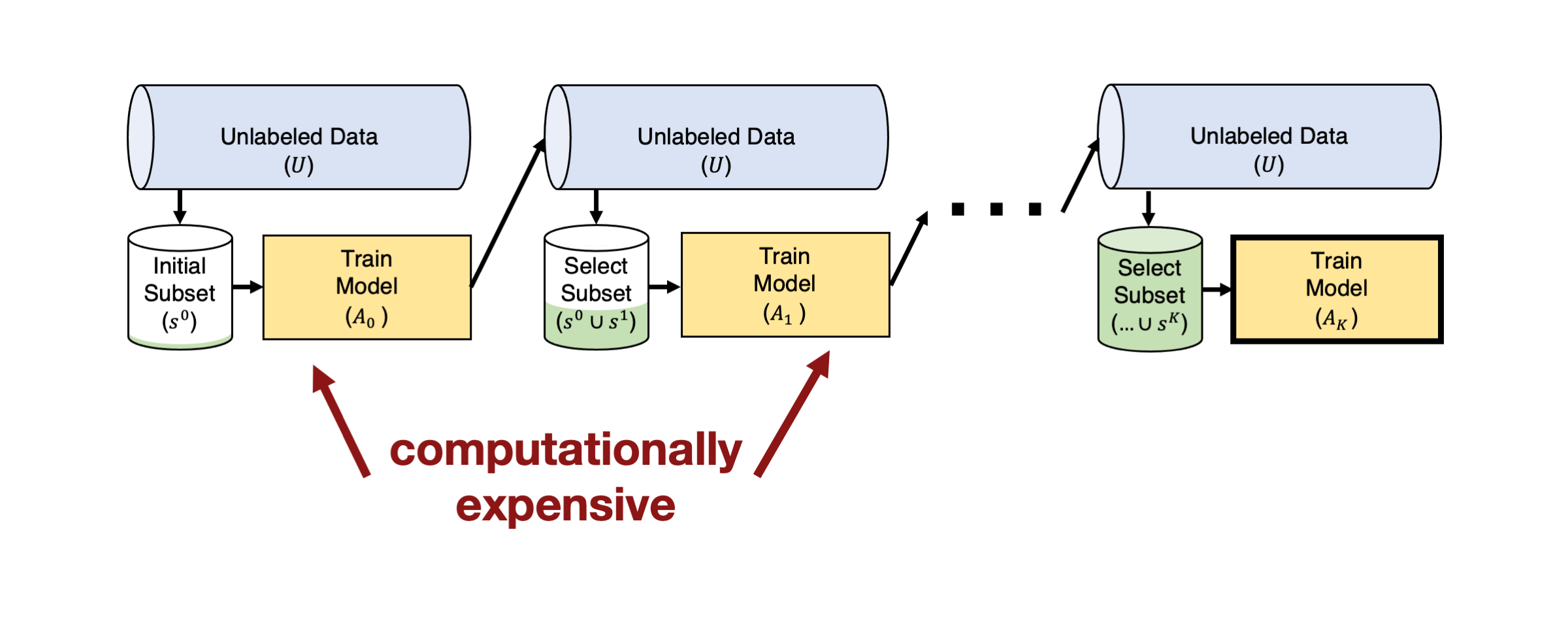
Practical Challenge 1: Big Models
Unfortunately, things are more challenging when we go from theory to practice. In modern ML, models used for image/text data have become quite large (with very high numbers of parameters). Here training the model each time we have collected more labels is computationally expensive.
In such settings, you can instead employ batch active learning, where we select a batch of examples to label in each round rather than only a single example. A simple approach to decide on a batch is merely to select the $J$ unlabeled examples with top values according to the acquisition function $ \phi(x, A_r)$ from above.
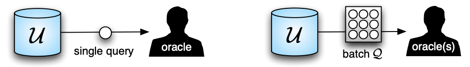
Figure from From Theories to Queries: Active Learning in Practice by Burr Settles.
However, this approach may fail to consider the diversity of the batch of examples being labeled next, because the acquisition function may take top values for unlabeled datapoints that all look similar. To ensure the batch of examples to label next are more representative of the remaining unlabeled pool, batch active learning strategies select $J$ examples with high information value that are also jointly diverse. For example, the greedy k-centers approach [S18] aims to find a small subset of examples that covers the dataset and minimizes the maximum distance from any unlabeled point to its closest labeled example.
Practical Challenge 2: Big Data
Active learning is also challenging with large amounts of unlabeled data, which has become commonplace in the era of big data. Many approaches search globally for the optimal examples to label and scale linearly or even quadratically with representation-based methods like the k-centers approach above. This quickly becomes intractable as we get to web-scale datasets with millions or billions of examples.
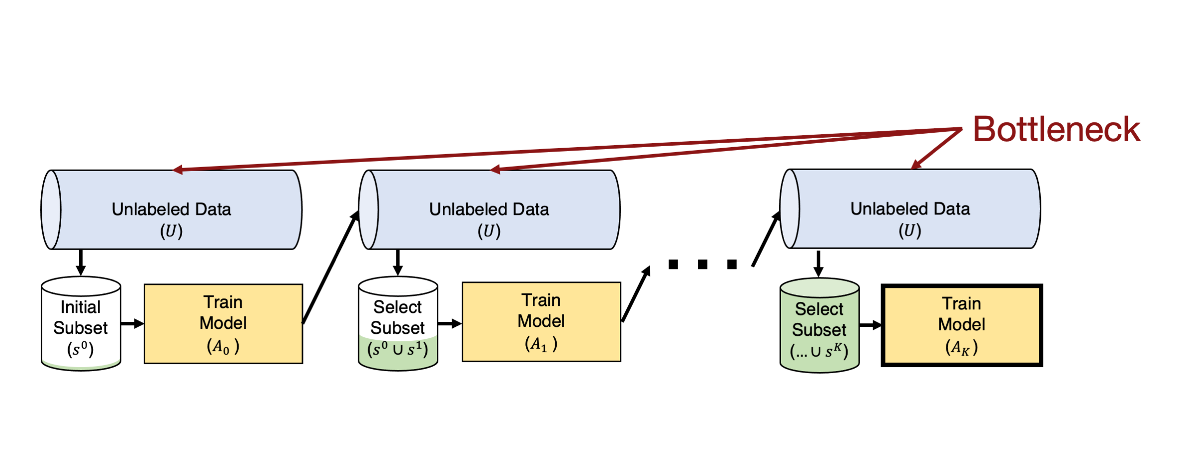
Luckily, one option to speed things up is to only compute the model outputs and acquisition function for a subset of the unlabeled pool. Many classes only make up a small fraction of the overall data in practice, and we can leverage the latent representations from pre-trained models to cluster these concepts. We can exploit this latent structure with methods like Similarity Search for Efficient Active Learning and Search of Rare Concepts (SEALS) [C22] to improve the computational efficiency of active learning methods by only considering the nearest neighbors of the currently labeled examples in each selection round rather than scanning over all of the unlabeled data.
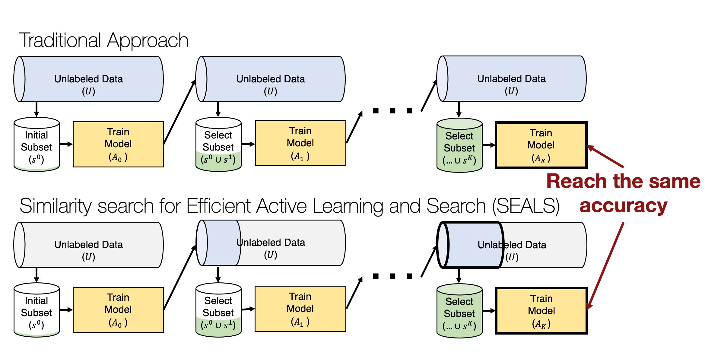
Finding the nearest neighbors for each labeled example in the unlabeled data can be performed efficiently with sublinear retrieval times [C02] and sub-second latency on datasets with millions or even billions of examples [J19]. While this restricted candidate pool of unlabeled examples impacts theoretical sample complexity, SEALS still achieves the optimal logarithmic dependence on the desired error for active learning. As a result, SEALS maintains similar label-efficiency and enables selection to scale with the size of the labeled data and only sublinearly with the size of the unlabeled data, making active learning and search tractable on web-scale datasets with billions of examples!
Core-set selection
What if we already have too much labeled data? Situations with systematic feedback (e.g., users tag their friends in photos or mark emails as spam) or self-supervision approaches like BERT [D19], SimCLR [CK20], and DINO [C21] can generate an unbounded amount of data. In these cases, processing all of the potential data would require a great deal of time and computational resources, which can be cumbersome or prohibitively expensive. This computation is often unnecessary because much of the data is redundant. This is where core-set selection helps.
The goal of core-set selection is to find a representative subset of data such that the quality of a model trained on the subset is similar or equivalent to the performance of training on the full data. The resulting core-set can dramatically reduce training time, energy, and computational costs.
There are a wide variety of core-set selection methods in the literature, but many of the techniques for core-set selection are dependent on the type of model and don’t generalize well to deep learning models. For example, the greedy k centers approach to core-set selection from above depends on the target model we want to train to quantify the distances between examples. Training the model to perform core-set selection would defeat the purpose and nullify any training time improvements we would get from reducing the data.
Luckily we don’t need to use the target model for the initial core-set selection process. Instead, we can make the selection with a smaller, less resource-hungry model, as proposed in Selection via Proxy [CY20]. For example, by simply reducing the number of layers in a model, we can create a proxy that is much faster to train but still provides a helpful signal for filtering data, leading to end-to-end training-time speed-ups:
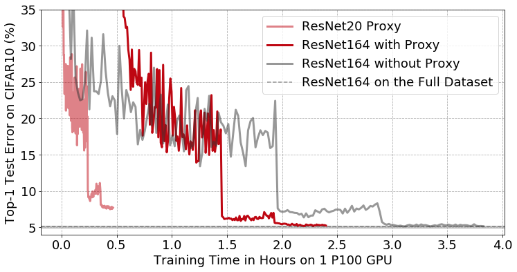
Training curves of a ResNet164 convolutional neural network classifier with pre-activation on CIFAR10 with and without data selection via proxy. The light red line shows training the proxy model (a smaller ResNet20 network). The solid red line shows training the target model (ResNet164) on a subset of images selected by the proxy. Using the proxy, we removed 50% of the data without impacting the final accuracy of ResNet164, reducing the end-to-end training time from 3 hours and 49 minutes to 2 hours and 23 minutes.
Lab
The lab assignments for the course are available in the dcai-lab repository.
Remember to run a git pull before doing every lab, to make sure you have the latest version of the labs.
The lab assignment for this lecture is in growing_datasets/Lab - Growing Datasets.ipynb. This lab guides you through an implementation of active learning.
References
[S18] Sener and Savarese. Active Learning for Convolutional Neural Networks: A Core-Set Approach. ICLR, 2018.
[C22] Coleman et al. Similarity Search for Efficient Active Learning and Search of Rare Concepts. AAAI, 2022.
[C02] Charikar. Similarity Estimation Techniques from Rounding Algorithms. STOC, 2002.
[J19] Johnson, Douze, Jégou. Billion-scale similarity search with GPUs. IEEE Transactions on Big Data, 2019.
[D19] Devlin et al. BERT: Pre-training of Deep Bidirectional Transformers for Language Understanding. NAACL-HLT, 2019.
[CK20] Chen et al. A Simple Framework for Contrastive Learning of Visual Representations. ICML, 2020.
[C21] Caron et al. Emerging Properties in Self-Supervised Vision Transformers. ICCV, 2021.
[CY20] Coleman et al. Selection via Proxy: Efficient Data Selection for Deep Learning. ICLR, 2020.
Licensed under CC BY-NC-SA.