Dataset Creation and Curation

Click here to view the raw lecture video on Panopto.
An edited version of this video will be posted after the course is over.

Creating a dataset for supervised learning requires the collection of examples and labels. This lecture will focus on classication tasks, but these ideas are applicable to other supervised learning tasks as well (regression, image segmentation, entity recognition, etc). This lecture covers three themes:

1. Concerns whether our ML task is properly framed to begin with (e.g. are we predicting appropriately defined classes in classification).

2. Concerns when sourcing data (e.g. selection bias).

3. Concerns when sourcing the labels (e.g. how to work with multiple data annotators and assess quality).

This lecture only covers a small part of complex topics like dataset collection/curation and labeling datasets with human workers. A more substantive overview is provided in the Human-in-the-Loop ML textbook [MM21].

Sourcing data

Key questions to ask when looking for training data include:

1. How will the resulting ML model be used? (On what population will the model be making predictions on and when)

2. What are hypothetical edge cases or high-stakes scenarios where we really need model make the right prediction?

Consider the following example from Beery et al. [BGP18]. The left-hand image is correctly predicted to contain a cow by a trained image classifier, whereas this model fails to produce the same prediction for the right-hand image. Can you say why?

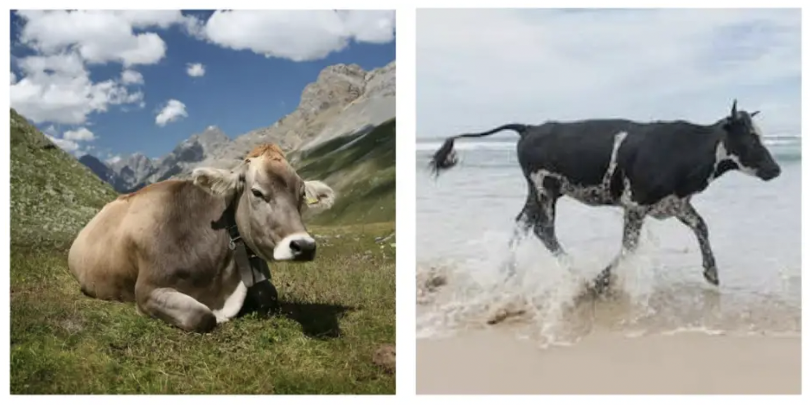
This is likely due to the fact that cows were always pictured in grass fields in the dataset used to train the classifier. When training models, we must always be aware of different types of correlations between features of the data and the labels. High-capacity ML models are like cheaters looking for shortcuts to their goal: they will try to exploit any correlation they can to produce high accuracy predictions on your dataset, even when these are spurious correlations that will fail to generalize when the model is deployed in the real-world.

Selection Bias

Spurious correlations can be present in a dataset due to selection bias [NBA17]. This refers to any systematic deviation between the distribution from which our collected training data stem and the actual distribution where the model will be deployed, i.e. our dataset fails to be representative of the real-world setting that we should care about. Also known as confounding or distribution shift, selection bias is extremely hard to account for via modeling, so always enumerate potential reasons for bias to creep into your data before collecting it.

Can you name common causes of selection bias?

• Time/location bias (e.g. training data collected in the past for applications where future data will look different, or collected from one country for a model deployed world-wide).

• Demographics bias (e.g. training data about people in which a particular minority group is under-represented).

• Response bias (e.g. survey response rates, prompting bias in the questions asked or multiple-choice answer options)

• Availability bias – using data that happens to be convenient rather than most representative (e.g. only surveying interviewees that are my friends).

• Long tail bias – in applications with many different possible rare scenarios, collection mechanisms may prevent some from appearing in the dataset (e.g. autonomous vehicle gets bumped into wrong side of road).

Dealing with selection bias in collected data

Once allowed to creep into your data, selection bias can be hard to mitigate via modeling. One strategy to at least better evaluate models trained on biased data is to hold out a validation set most representative of conditions expected during deployment:

• If data are collected over time in a changing environment, one might hold out the most recent data as the validation set.
• If data are collected from multiple locations and new locations will be encountered during deployment, one might reserve all data from some locations for validation.
• If data contain important but rare events, one might over-sample these when randomly selecting validation data.

How much data will we need to collect?

Consider an application where you want to train a classifier to achieve at least 95% accuracy. How much data should you collect to achieve this? What is the value of collecting additional data (how much further do we expect accuracy to improve)?

Here is a simple method to estimate this, assuming we already have some training data $D_\text{train}$ of sample size $n$ and a separate fixed size validation dataset $D_\text{val}$. First decide on grid of random data subsets of say sizes: $n_1 = 0.1 \cdot n, n_2 = 0.2 \cdot n, n_3 = 0.3 \cdot n, …, n_{10} = 1 \cdot n$. Then:

For $j = 1,\dots, 10$:

This produces a small set of pairs $ \{ (n_j, a_{ij}) \}$. Using this set, our goal is to predict what the accuracy $a’$ would be for a model trained on dataset of much larger sample size $n’ \gg n$ than our original training data $D_\text{train}$. Can you guess why using a K Nearest Neighbor or Linear Regression model to do this prediction is a bad idea?

The task of predicting accuracy at $n’$ requires extrapolation, which is one area where we definitely need to be model-centric (since the nature of extrapolation means there is little relevant data to begin with). Here we can rely on an empirical observation [RRB20] that the performance of a model is remarkably predictable according to:

\[\log (\text{error}) = - a \cdot \log (n) + b\]

We can estimate the scalar parameters $a, b$ of this simple model by minimizing the mean squared error over observations $ \{ (n_j, 1 - a_{ij}) \}$. Subsequently just plug in $n’$ to the above formula to predict the error expected for a model trained on a larger dataset of this size.

For small datasets without a pre-defined validation split, you can alternatively use cross-validation to get more stable measurements of $a_{ij}$ on subsets of the dataset.

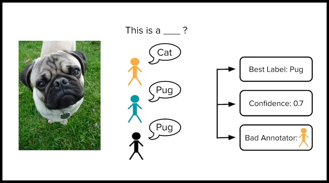
Labeling data with crowdsourced workers

Many supervised learning datasets must be annotated by human workers to get labels for training models. For instance, medical images of tumors may be labeled by a team of doctors as cancerous vs benign. Because individual doctors can make mistakes, we can obtain more reliable labels by having multiple doctors independently annotate an image.

Concretely, suppose we have a classification dataset of $n$ examples labeled by $J$ annotators, where $Y_{ij} \in \{1,2,…,K\}$ denotes the class that annotator $j$ chose for example $i$. While we’d like every annotator to label every example, this is often infeasible, and we thus let $Y_{ij} = \emptyset$ if annotator $j$ did not label example $i$. Some examples may be labeled by multiple annotators, and to most wisely allocate labeling efforts, we’d like to collect more annotations for harder examples than easier ones.

Can you identify potential concerns when crowdsourcing labels in this manner?

1. Some annotators may provide less accurate labels than other annotators.
2. Some annotators may collude with other annotators (copying their choices whether right or wrong).

The gold standard way to diagnose such problems is to slip a few “quality control” examples into the dataset, for which we already know the ground-truth label. The subset of data provided to each annotator for labeling should contain some quality control examples.

Curating a dataset labeled by multiple annotators

Unfortunately many datasets labeled by multiple annotators did not contain quality control examples. Given such a dataset, here we consider how to estimate three quantities:

1. A consensus label for each example that aggregates the individual annotations.
2. A quality score for each consensus label which measures our confidence that this label is correct.
3. A quality score for each annotator which estimates the overall correctness of their labels.

We consider three algorithms to estimate 1-3 above: Majority Vote + Inter-Annotator Agreement, Dawid-Skene, and CROWDLAB.

Majority Vote and Inter-Annotator Agreement

The simplest way to establish a consensus label $\widehat{Y}_i$ for example $i$ is to take a majority vote amongst all the available annotations $\{ Y_{ij}\}_{j \in \mathcal{J}_i}$ for this example. Here $\mathcal{J}_i = \{j : Y_{ij} \neq \emptyset \}$ denotes the subset of annotators that labeled example $i$.

One can quantify the confidence that this consensus label is correct via the agreement between annotations for this example:

\[\text{Agreement}_i = \frac{1}{| \mathcal{J}_i |} \sum_{j \in \mathcal{J}_i} \big[ Y_{ij} == \widehat{Y}_i \big]\]

One can estimate the overall quality of annotator $j$ based on the fraction of their annotations that agree with the consensus label for the same example:

\[\text{Quality}_j = \frac{1}{| \mathcal{I}_{j,+} |} \sum_{i \in \mathcal{I}_{j,+}} \big[ Y_{ij} == \widehat{Y}_i \big]\]

where $\mathcal{I}_j = \{ i \in [n] : Y_{ij} \neq \emptyset \}$ denotes the subset of examples labeled by annotator $j$, and $\mathcal{I}_{j,+} = \{i \in \mathcal{I}_j : |\mathcal{J}_i| > 1 \}$ is the subset of these that are also labeled by at least one other annotator. Note that we should not evaluate labels from annotator $j$ against the consensus label for examples which were only labeled by annotator $j$.

Can you list downsides of producing estimates like this?

1. Resolving ties is ambiguous in majority vote.
2. A bad annotator and good annotator have equal impact on the estimates.

Dawid-Skene

To address the above concerns, one can instead assume a statistical generative process to analyze multi-annotator classification data [PCC18]. A popular choice is Dawid-Skene, which parameterizes each annotator $j$ via a matrix $\mathbf{C}_j \in \mathbb{R}^{K \times K}$ whose entries $\mathbf{C}_j^{a,b}$ are the probability that annotator $j$ mislabels an example as class $b$ when it actually belongs to class $a$. With an appropriate joint Dirichlet prior distribution placed upon them, the collection of parameters $\{ \mathbf{C}_j \}$ can be estimated from the data via Bayesian inference. This is commonly approximated through MAP inference to maximize the likelihood of the observed annotations $\{ Y_{ij} \}$ via the Expectation-Maximization algorithm.

Subsequently, the quality of annotator $j$ can be estimated via: $\text{Trace}(\mathbf{C}_j)$.
When the $\mathbf{C}_j$ are well-estimated and assumptions of Dawid-Skene are satisified by the real data, then an annotator who tends to make less mistakes should have larger values along the diagonal of $\mathbf{C}_j$.

Assuming some prior distribution over the classes $\pi_Y$ (e.g. chosen proportional to their observed frequencies in the dataset), a posterior distribution for the true label of example $i$ is estimated via: \(\Pr(Y_i = k) \propto \pi_Y \cdot \prod_{j \in \mathcal{J}_i} \mathbf{C}_j^{k,Y_{ij}}\)
This posterior will be more concentrated around one class for examples that are labeled by many annotators, where each annotator agrees with the others and is estimated to be a high-quality annotator.

From this posterior, a consensus label can be estimated as:

\[\widehat{Y}_i = \arg\max_k \Pr(Y_i = k)\]

Our confidence that $\widehat{Y}_i$ matches the true label can be estimated via: $\Pr(Y_i = \widehat{Y}_i)$

Downsides of Dawid-Skene include:

1. Strong assumptions which ignore how labels are related to features of the examples.

2. If annotators provide noisy labels, Dawid-Skene cannot establish reliable consensus for examples only labeled by a single annotator.

3. Dawid-Skene must estimate many parameters, an entire $K \times K$ matrix ($K$ being the number of classes) for every annotator. This is statistically challenging with limited data, particularly if some annotators labeled few examples or did not overlap much other annotators.

CROWDLAB (Classifier Refinement Of croWDsourced LABels)

If we also want to account for feature values measured for each example (upon which the crowdsourced labels are anyway based), a natural way is to train a classification model to predict the labels for any example. Such a model $M$ can be trained with consensus labels derived via any method, such as simple majority-vote.

CROWDLAB combines probabilistic predictions from the classifier with the annotations to estimate consensus labels and their quality [GTM22]. CROWDLAB estimates are based on the intuition that we should rely on the classifier’s prediction more for examples that are labeled by few annotators but less for examples labeled by many annotators (with many annotations, simple agreement already provides a good confidence measure). If we have trained a good classifier, we should rely on it more heavily but less so if its predictions appear less trustworthy. Generalizing across the feature space, a good classifier can to produce an accurate prediction for an example labeled by a single annotator. This may help better assess whether this single annotation is reliable or not.

CROWDLAB relies on predicted class probabilities from any trained classifier model: $p_M = \widehat{p}_M(Y_i \mid X_i)$. These are ideally held-out predictions produced for each example in a dataset via cross-validation. For a particular example $i$, we form an analogous “predicted” class probability vector $p_j$ based on the annotation $Y_{ij}$ from each annotator that labeled this example. Like Dawid-Skene, CROWDLAB estimates a distribution for the true label of example $i$. However it does this via a simple weighted combination: \(\Pr(Y_i) = \frac{1}{Z} (w_M \cdot p_M + \sum_{j \in \mathcal{J}_i} w_j \cdot p_j )\)

Here $Z = w_M + \sum_{j \in \mathcal{J}_i} w_j$ and global weights $w_M, w_1, …, w_J$ are estimates of how trustworthy the model is vs. each individual annotator. The same weights are used for all examples. Adaptive weighting allows CROWDLAB to still perform effectively even when the classifier is suboptimal or a few of the annotators often give incorrect labels. We compute a consensus label and confidence score for its correctness from $\Pr(Y_i)$ as we did for Dawid-Skene above.

Intuitively, the weighted ensemble prediction for a particular example becomes more heavily influenced by the annotators the more of them have labeled this example. The inter-annotator agreement should serve as a good proxy for consensus label quality when many annotators were involved, whereas this quantity is unreliable for examples labeled by few annotators, for which CROWDLAB relies more on the classifier (which can generalize to these examples if there were other examples with similar feature values in the dataset). CROWDLAB also accounts for the classifier’s prediction confidence, its accuracy against the annotators, and per-annotator deviations from the majority to even better assess which estimates are least reliable.

Details to estimate weights

Let $s_j$ represent annotator $j$’s agreement with other annotators who labeled the same examples.

\[s_j = \frac{\sum_{i \in \mathcal{I}_j} \sum_{\ell \in \mathcal{J}_i, \ell \neq j} [Y_{ij} == Y_{i\ell}]}{\sum_{i \in \mathcal{I}_j} ( |\mathcal{J}_i| -1 )}\]

Let $A_{M}$ be the (empirical) accuracy of our classifier with respect to the majority-vote consensus labels over the examples with more than one annotation (for which consensus is more trustworthy).

\[A_{M} = \frac{1}{|\mathcal{I}_+|} \sum_{i \in \mathcal{I}_+} \big[ Y_{i,M} == \widehat{Y_i} \big] \label{eq:am}\]

Here $Y_{i,M} \in \{1,2,…,K\}$ is the class predicted by our model for $X_i$. To normalize against a baseline, we calculate the accuracy $A_{\text{MLC}}$ of always predicting the most common overall class $Y_{\text{MLC}}$, which is the class selected the most overall by the annotators. This accuracy is also calculated on the subset of examples that have more than one annotator $\mathcal{I}_+$.

\[A_{\text{MLC}} = \frac{1}{|\mathcal{I}_+|} \sum_{i \in \mathcal{I}_+} \big[ Y_{\text{MLC}} = \widehat{Y_i} \big]\]

Based on this majority-class-accuracy baseline, we choose our weights to be baseline-normalized versions of: each annotator’s overall agreement with other annotators, and the overall accuracy of the model.

\[w_j = 1 - \frac{1 - s_j}{1 - A_{\text{MLC}}}\] \[w_{\mathcal{M}} = \left( 1 - \frac{1 - A_{\mathcal{M}}}{1 - A_{\text{MLC}}} \right) \cdot \sqrt{\frac{1}{n} \sum_i |\mathcal{J}_i|}\]

Details to estimate $p_j$

Rather than directly including the class annotations (as in majority-vote), CROWDLAB first converts each annotation to a corresponding predicted class probability vector $p_j$ for example $i$. This allows for the possibility of annotation error. To quantify this possibility, we define a likelihood parameter $P$ set as the average annotator agreement, across examples that have more than one annotation. $P$ estimates the probability that an arbitrary annotator’s label will match the majority-vote consensus label for an arbitrary example.

\[P = \frac{1}{|\mathcal{I}_+|} \sum_{i \in \mathcal{I}_+} \frac{1}{| \mathcal{J}_i |} \sum_{j \in \mathcal{J}_i} \big[ Y_{ij} = \widehat{Y}_i \big]\]

Here $\mathcal{I}_{+} = \{i = 1,…,n : |\mathcal{J}_i| > 1 \}$ are the examples with multiple annotations.

We then simply define our predicted class probability vector $p_j$ (corresponding to the label annotator $j$ chose for example $i$) to be:

\[p_j = \begin{cases} P & \mbox{when } Y_{ij} = k\\ \frac{1 - P}{K - 1} & \mbox{when } Y_{ij} \neq k \end{cases}\]

This simple likelihood is shared across annotators and only involves a single shared parameter $P$ that is easily estimated from the data.

Estimating annotator quality

CROWDLAB uses a similar weighted aggregation to estimate the overall quality of each annotator. Here the annotator’s deviations from consensus labels are adjusted by our confidence in these consensus labels based in part on the classifier’s probabilistic predictions. See the CROWDLAB paper for details [GTM22].

Lab

A hands-on lab assignment to accompany this lecture is available in the dcai-lab repository. The assignment, found in the notebook dataset_curation/Lab – Dataset Curation with Multiple Annotators, is to analyze an already collected dataset labeled by multiple annotators.

References

[MM21] Munro, R., Monarch, R. Human-in-the-Loop Machine Learning: Active Learning and Annotation for Human-centered AI. 2021.

[GTM22] Goh, H. W., Tkachenko, U., and Mueller, J. CROWDLAB: Supervised learning to infer consensus labels and quality scores for data with multiple annotators. NeurIPS 2022 Human in the Loop Learning Workshop, 2022.

[PCC18] Paun, S., et al. Comparing Bayesian Models of Annotation. Transactions of the Association for Computational Linguistics, 2018.

[NBA17] Nunan, D., Bankhead, C., Aronson J. K. Catalogue of Bias, 2017.

[BGP18] Beery, S., Van Horn, G., and Perona, P. Recognition in terra incognita. European Conference on Computer Vision, 2018.

[RRB20] Rosenfeld, J., Rosenfeld, A., and Belinkov, Y. A constructive prediction of the generalization error across scales. International Conference on Learning Representations, 2020.

[LTH22] Liang, W., et al. Advances, challenges and opportunities in creating data for trustworthy AI. Nature Machine Intelligence, 2022.

---