Label Errors and Confident Learning

Click here to view the raw lecture video on Panopto.
An edited version of this video will be posted after the course is over.

Slides: [pdf, pptx]

If you’ve ever used datasets like CIFAR, MNIST, ImageNet, or IMDB, you likely assumed the class labels are correct. Surprise: there are 100,000+ label issues in ImageNet. In this lecture, we introduce a principled and theoretically grounded framework called confident learning (open-sourced in the cleanlab package) that can be used to identify label issues/errors, characterize label noise, and learn with noisy labels automatically for most classification datasets.

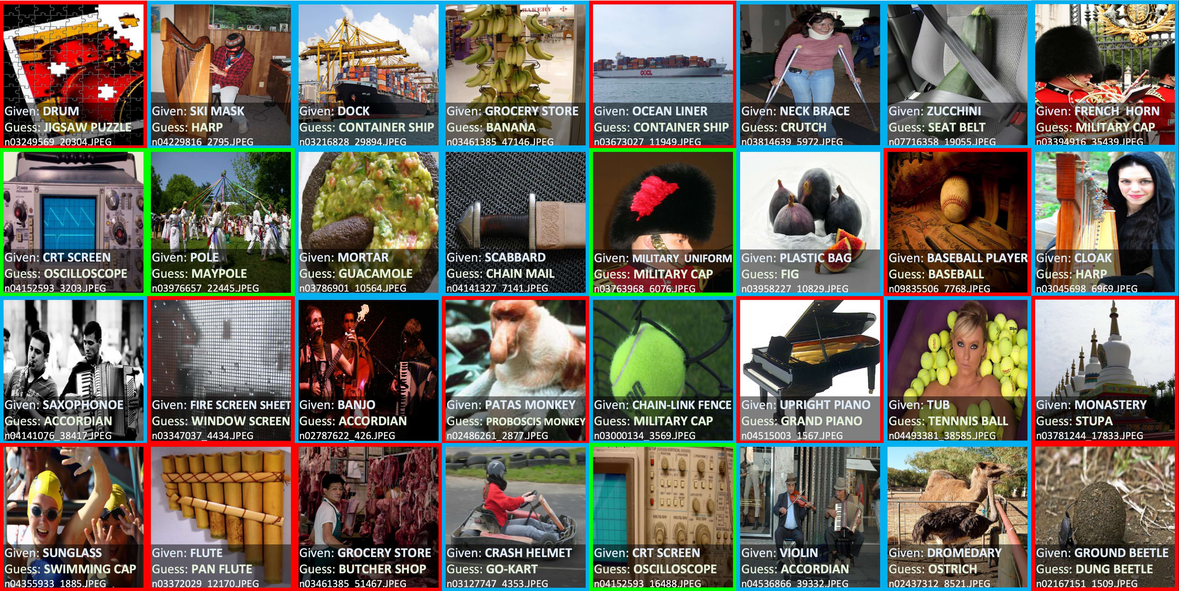
Top 32 label issues in the 2012 ILSVRC ImageNet train set identified using confident learning. Label Errors are boxed in red. Ontological issues in green. Multi-label images in blue.

The figure above shows examples of label errors in the 2012 ILSVRC ImageNet training set found using confident learning. For interpretability, we group label issues found in ImageNet using CL into three categories:

1. Multi-label images (blue) have more than one label in the image.
2. Ontological issues (green) comprise is-a (bathtub labeled tub) or has-a (oscilloscope labeled CRT screen) relationships. In these cases, the dataset should include one of the classes.
3. Label errors (red) occur when a class exists in the dataset that is more appropriate for an example than its given class label.

Using confident learning, we can find label errors in any dataset using any appropriate model for that dataset. Here are three other real-world examples in common datasets.

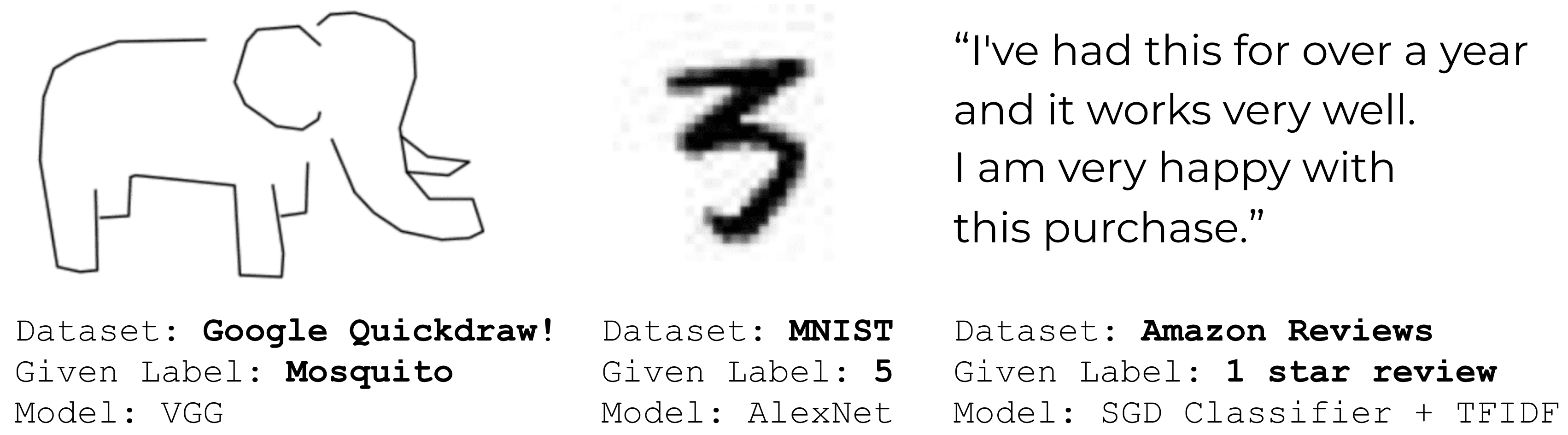
Examples of label errors that currently exist in Amazon Reviews, MNIST, and Quickdraw datasets identified using confident learning for varying data modalities and models.

What is Confident Learning?

Confident learning (CL) has emerged as a subfield within supervised learning and weak-supervision to:

• characterize label noise
• find label errors
• learn with noisy labels
• find ontological issues

CL is based on the principles of pruning noisy data (as opposed to fixing label errors or modifying the loss function), counting to estimate noise (as opposed to jointly learning noise rates during training), and ranking examples to train with confidence (as opposed to weighting by exact probabilities). Here, we generalize CL, building on the assumption of Angluin and Laird’s classification noise process , to directly estimate the joint distribution between noisy (given) labels and uncorrupted (unknown) labels.

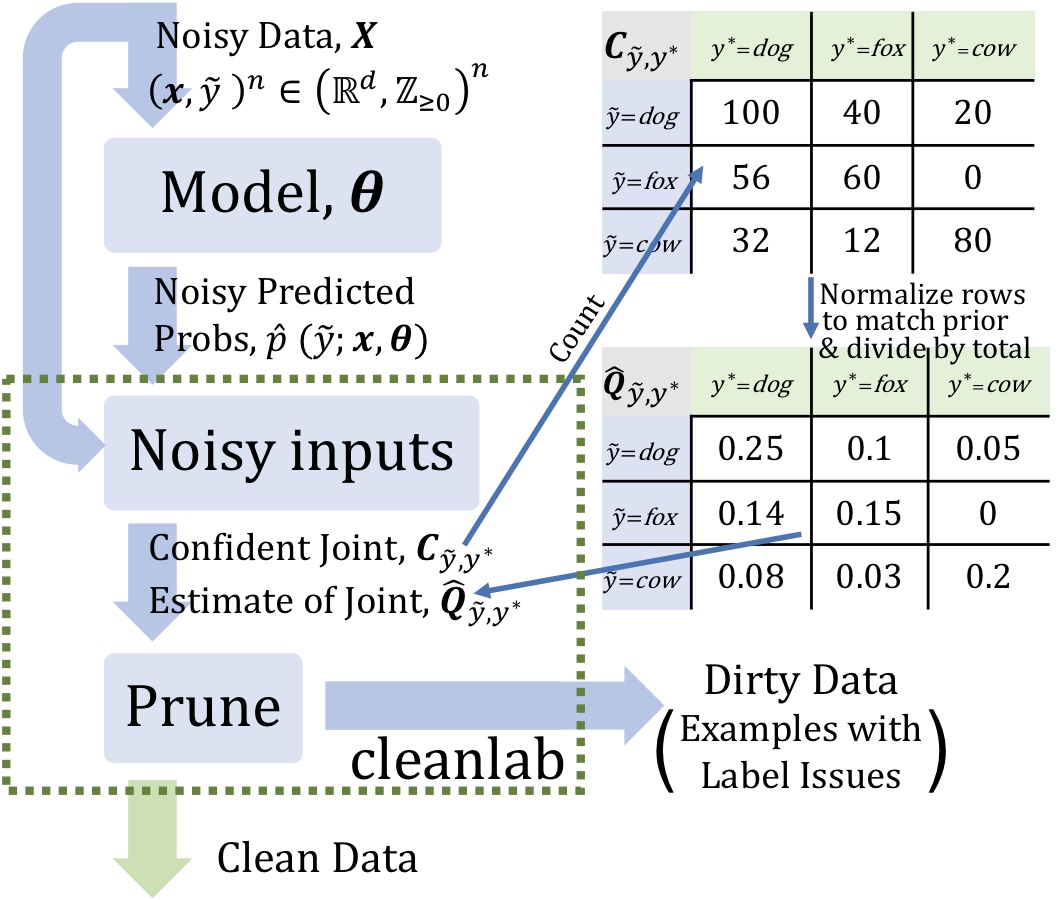
The confident learning process and examples of the confident joint and estimated joint distribution between noisy (given) labels and uncorrupted (unknown) labels. \(\tilde{y}\) denotes an observed noisy label and \(y^*\) denotes a latent uncorrupted label.

From the figure above, we see that CL requires two inputs:

• out-of-sample predicted probabilities (matrix size: # of examples by # of classes)
• noisy labels (vector length: number of examples)

For the purpose of weak supervision, CL consists of three steps:

1. Estimate the joint distribution of given, noisy labels and latent (unknown) uncorrupted labels to fully characterize class-conditional label noise.
2. Find and prune noisy examples with label issues.
3. Train with errors removed, re-weighting examples by the estimated latent prior.

Benefits of Confident Learning

Unlike most machine learning approaches, confident learning requires no hyperparameters. We use cross-validation to obtain predicted probabilities out-of-sample. Confident learning features a number of other benefits. CL

• directly estimates the joint distribution of noisy and true labels
• works for multi-class datasets
• finds the label errors (errors are ordered from most likely to least likely)
• is non-iterative (finding training label errors in ImageNet takes 3 minutes)
• is theoretically justified (realistic conditions exactly find label errors and consistent estimation of the joint distribution)
• does not assume randomly uniform label noise (often unrealistic in practice)
• only requires predicted probabilities and noisy labels (any model can be used)
• does not require any true (guaranteed uncorrupted) labels
• extends naturally to multi-label datasets
• is free and open-sourced as the cleanlab Python package for characterizing, finding, and learning with label errors.

The Principles of Confident Learning

CL builds on principles developed across the literature dealing with noisy labels:

• Prune to search for label errors, e.g. following the example of Natarajan et al. (2013); van Rooyen et al. (2015); Patrini et al. (2017), using soft-pruning via loss-reweighting, to avoid the convergence pitfalls of iterative re-labeling.
• Count to train on clean data, avoiding error-propagation in learned model weights from reweighting the loss (Natarajan et al., 2017) with imperfect predicted probabilities, generalizing seminal work Forman (2005, 2008); Lipton et al. (2018).
• Rank which examples to use during training, to allow learning with unnormalized probabilities or SVM decision boundary distances, building on well-known robustness findings of PageRank (Page et al., 1997) and ideas of curriculum learning in MentorNet (Jiang et al.,2018).

Theoretical Findings in Confident Learning

For full coverage of CL algorithms, theory, and proofs, please read our paper. Here, I summarize the main ideas.

Theoretically, we show realistic conditions where CL (Theorem 2: General Per-Example Robustness) exactly finds label errors and consistently estimates the joint distribution of noisy and true labels. Our conditions allow for error in predicted probabilities for every example and every class.

How does Confident Learning Work?

To understand how CL works, let’s imagine we have a dataset with images of dogs, foxes, and cows. CL works by estimating the joint distribution of noisy and true labels (the Q matrix on the right in the figure below).

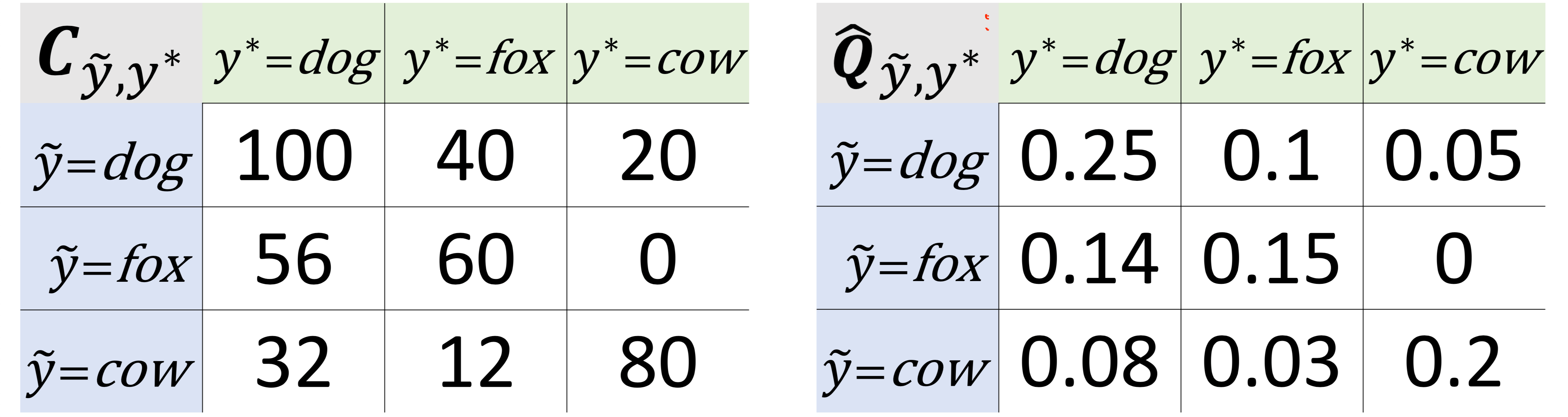
Left: Example of confident counting examples. This is an unnormalized estimate of the joint. Right: Example joint distribution of noisy and true labels for a dataset with three classes.

Continuing with our example, CL counts 100 images labeled dog with high probability of belonging to class dog, shown by the C matrix in the left of the figure above. CL also counts 56 images labeled fox with high probability of belonging to class dog and 32 images labeled cow with high probability of belonging to class dog.

For the mathematically curious, this counting process takes the following form.

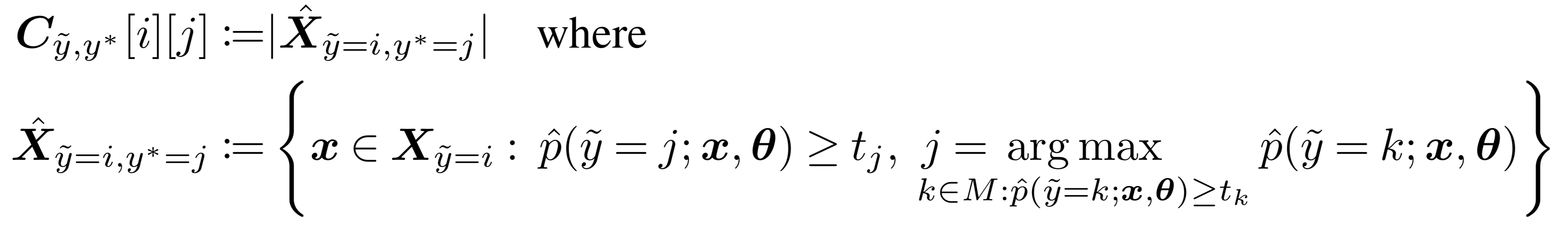
For an in-depth explanation of the notation, check out the CL paper. The central idea is that when the predicted probability of an example is greater than a per-class-threshold, we confidently count that example as actually belonging to that threshold’s class. The thresholds for each class are the average predicted probability of examples in that class. This form of thresholding generalizes well-known robustness results in PU Learning (Elkan & Noto, 2008) to multi-class weak supervision.

Find label issues using the joint distribution of label noise

From the matrix on the right in the figure above, to estimate label issues:

1. Multiply the joint distribution matrix by the number of examples. Let’s assume 100 examples in our dataset. So, by the figure above (Q matrix on the right), there are 10 images labeled dog that are actually images of foxes.
2. Mark the 10 images labeled dog with largest probability of belonging to class fox as label issues.
3. Repeat for all non-diagonal entries in the matrix.

Note: this simplifies the methods used in our paper, but captures the essence.

Practical Applications of Confident Learning

CL Improves State-of-the-Art in Learning with Noisy Labels by over 10% on average and by over 30% in high noise and high sparsity regimes

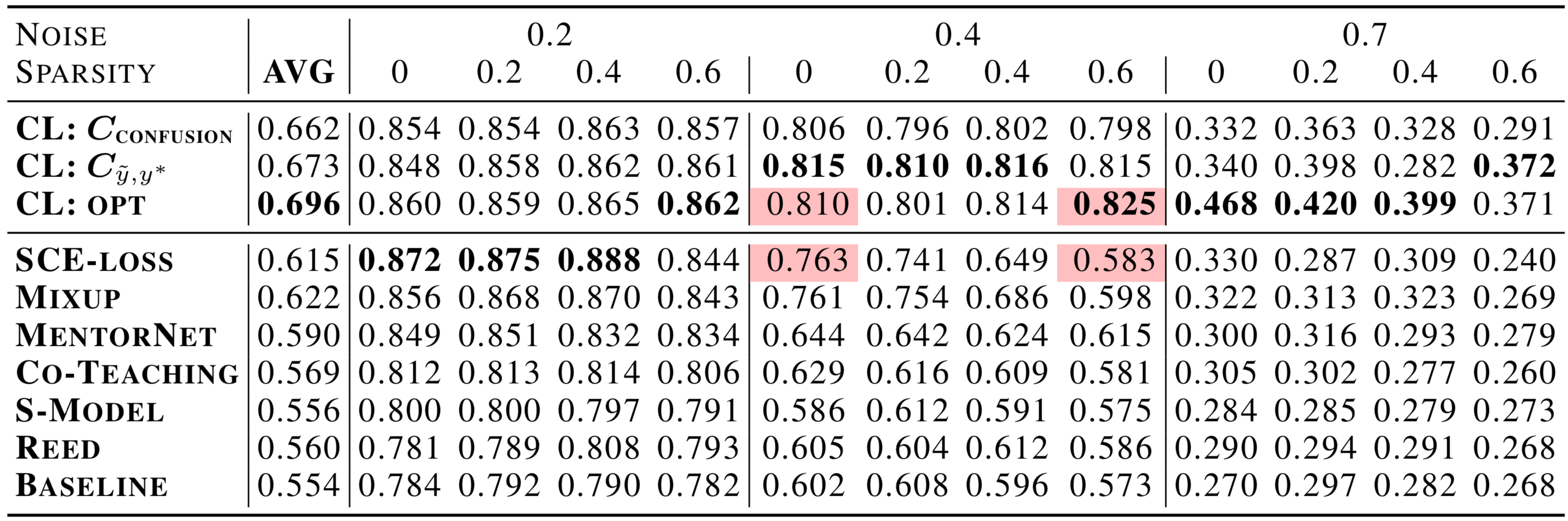
The table above shows a comparison of CL versus recent state-of-the-art approaches for multiclass learning with noisy labels on CIFAR-10. At high sparsity (see next paragraph) and 40% and 70% label noise, CL outperforms Google’s top-performing MentorNet, Co-Teaching, and Facebook Research’s Mix-up by over 30%. Prior to confident learning, improvements on this benchmark were significantly smaller (on the order of a few percentage points).

Sparsity (the fraction of zeros in Q) encapsulates the notion that real-world datasets like ImageNet have classes that are unlikely to be mislabeled as other classes, e.g. p(tiger,oscilloscope) ~ 0 in Q. Shown by the highlighted cells in the table above, CL exhibits significantly increased robustness to sparsity compared to state-of-the-art methods like Mixup, MentorNet, SCE-loss, and Co-Teaching. This robustness comes from directly modeling Q, the joint distribution of noisy and true labels.

Training on ImageNet cleaned with CL Improves ResNet Test Accuracy

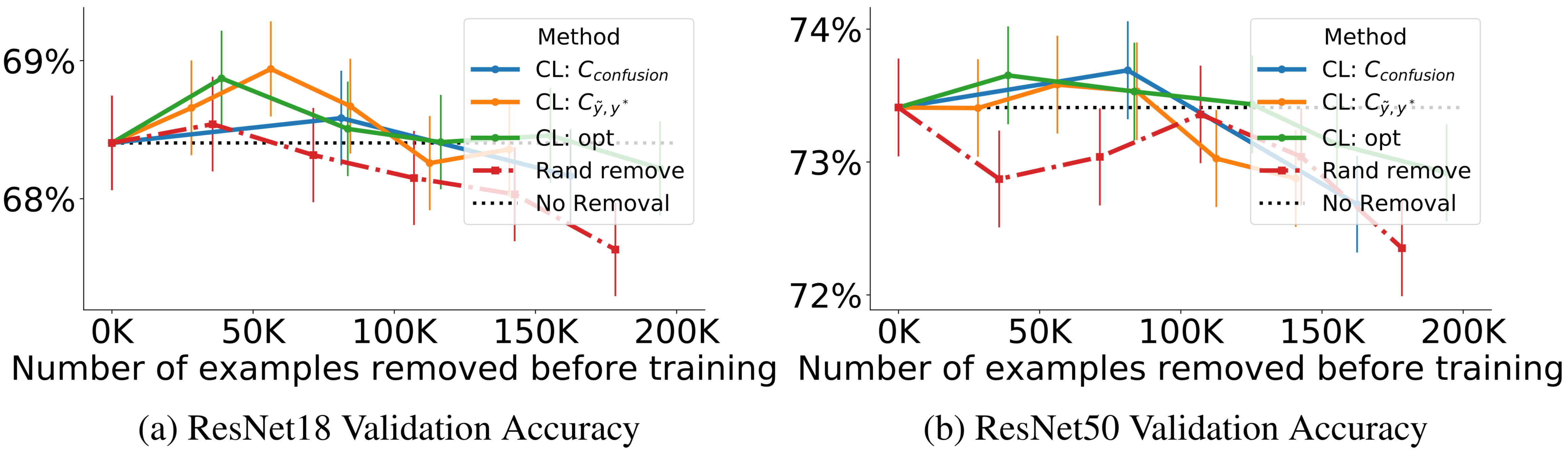
In the figure above, each point on the line for each method, from left to right, depicts the accuracy of training with 20%, 40%…, 100% of estimated label errors removed. The black dotted line depicts accuracy when training with all examples. Observe increased ResNet validation accuracy using CL to train on a cleaned ImageNet train set (no synthetic noise added) when less than 100k training examples are removed. When over 100k training examples are removed, observe the relative improvement using CL versus random removal, shown by the red dash-dotted line.

Good Characterization of Label Noise in CIFAR with Added Label Noise

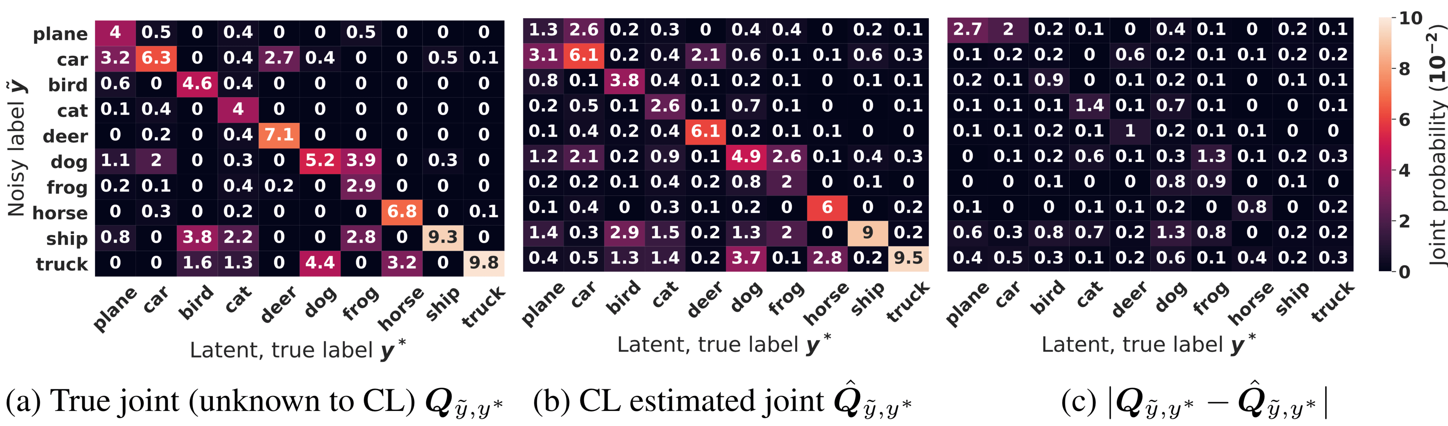
The figure above shows CL estimation of the joint distribution of label noise for CIFAR with 40% added label noise. Observe how close the CL estimate in (b) is to the true distribution in (a) and the low error of the absolute difference of every entry in the matrix in (c). Probabilities are scaled up by 100.

Automatic Discovery of Onotological (Class-Naming) Issues in ImageNet

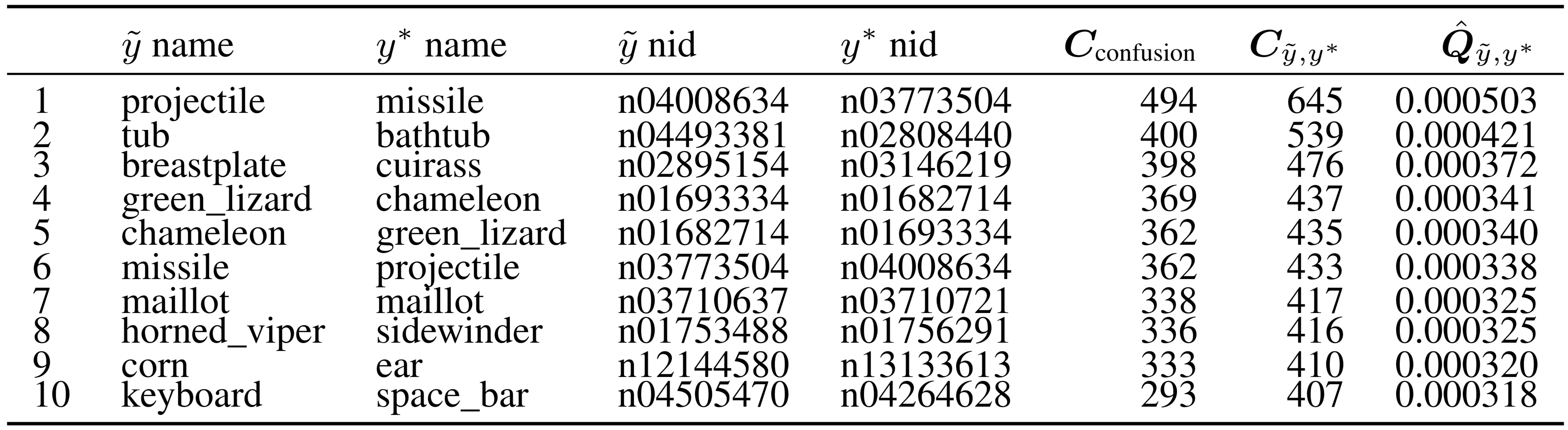
CL automatically discovers ontological issues of classes in a dataset by estimating the joint distribution of label noise directly. In the table above, we show the largest off diagonals in our estimate of the joint distribution of label noise for ImageNet, a single-class dataset. Each row lists the noisy label, true label, image id, counts, and joint probability. Because these are off-diagonals, the noisy class and true class must be different, but in row 7, we see ImageNet actually has two different classes that are both called maillot. Also observe the existence of misnomers: projectile and missile in row 1, is-a relationships: bathtub is a tub in row 2, and issues caused by words with multiple definitions: corn and ear in row 9.

Final Thoughts

Our theoretical and experimental results emphasize the practical nature of confident learning, e.g. identifying numerous label issues in ImageNet and CIFAR and improving standard ResNet performance by training on a cleaned dataset. Confident learning motivates the need for further understanding of uncertainty estimation in dataset labels, methods to clean training and test sets, and approaches to identify ontological and label issues in datasets.

Resources

• This lecture overviews the paper (JAIR 2021) Confident Learning: Estimating Uncertainty in Dataset Labels
• This lecture also covers the label errors paper (NeurIPS 2021): Pervasive Label Errors in Test Sets Destabilize Machine Learning Benchmarks
• Results of this method on the ten most commonly cited test sets in ML: https://labelerrors.com
• Try these methods yourself (open-sourced via cleanlab): https://github.com/cleanlab/cleanlab.
• The cleanlab package is a data-centric AI package for improving ML models by improving datasets and supports things like training ML models and deep learning models with noisy labels, outliers, and data labeled by multiple annotators. Learn more in the cleanlab documentation. cleanlab + the confidentlearning-reproduce repo reproduces results in the CL paper.

Lab

The lab assignments for the course are available in the dcai-lab repository.

Remember to run a git pull before doing every lab, to make sure you have the latest version of the labs.

The lab assignment for this class is in label_errors/Lab - Label Errors.ipynb. This lab guides you through writing your own implementation of automatic label error identification using Confident Learning, the technique taught in today’s lecture.

---