Data-centric Evaluation of ML Models
Most Machine Learning applications involve these steps:
- Collect data and define the appropriate ML task for your application.
- Explore the data to see if it exhibits any fundamental problems.
- Preprocess the data into a format suitable for ML modeling.
- Train a straightforward ML model that is expected to perform reasonably.
- Investigate shortcomings of the model and the dataset.
- Improve the dataset to address its shortcomings.
- Improve the model (architecture search, regularization, hyperparameter tuning, ensembling different models).
- Deploy model and monitor subsequent data for new issues.
This lecture will focus on step 5, the foundation for improving ML performance. Topics covered include:
- Evaluation of ML models (a prerequisite for improving them).
- Handling poor model performance for some particular subpopulation.
- Measuring the influence of individual datapoints on the model.
A Recap of Multi-class Classification
Here we focus on classification tasks, although the same ideas presented in this lecture are applicable to other supervised learning tasks as well. Let’s quickly recap the standard classification setting with $K$ classes [R08, HTF17].
In classification, we have a training dataset $\mathcal{D}$ with $n$ examples: $(x_i, y_i) \sim P_{XY}$ sampled from some underlying distribution (a.k.a. population) over features $X$ and class labels $Y$. Here $y_i \in \{1, 2, \dots, K\}$ denotes the class label of the $i$th example (one of $K$ possible classes) and $x_i$ are some feature measurements used to represent the $i$th example (e.g. pixel intensities of an image).
Goal: Use $\mathcal{D}$ to train a model $M$, which given an example with new feature values $x$, produces a vector of predicted class probabilities $M(x) = [p_1,\dots, p_K]$ whose $k$th entry approximates $P(Y = k \mid X = x)$.
For a particular loss function that scores each model prediction, we seek a model $M$ that optimizes:
\[\min_M \ \mathbb{E}_{(x,y) \sim P_{XY}} \ \big[ \text{Loss}\big(M(x), y \big) \big]\]Key assumptions:
- Data encountered during deployment will stem from the same distribution $P_{XY}$ as our training data $\mathcal{D}$.
- Training data $(x_i, y_i)$ are independent and identically distributed (IID).
- Each example belongs to exactly one class.
In practice always consider:
- including an “Other” class and redefining your classes to be more disjoint if worried that two classes may both be appropriate for some examples (e.g. “laptop” and “computer”).
- whether the ordering of your data matters.
Evaluation of ML models
We use the Loss function to evaluate model predictions for a new example $x$ against its given label $y$ [Z15, VC22]. The loss may be a function of either:
-
The predicted class $\hat{y} \in \{1,2, \dots, K\}$ deemed most likely for $x$. Examples of such classification losses include: accuracy, balanced accuracy, precision, recall,… These measure how often the class prediction from our model matches the observed label, and directly evaluate decisions made based on the model.
-
The predicted probabilities $[p_1, p_2, \dots, p_K] \in \mathbb{R}^K$ of each class for $x$. Examples of such classification losses include: log loss, AUROC, calibration error,… These measure how well the model estimates the proportion of times the observed label $y$ would take each class value, in a hypothetical experiment in which many examples with the same feature values $x$ could be sampled repeatedly. Predicted class probabilities are especially useful to determine optimal decisions from classifier outputs in asymmetric reward settings (e.g. if placing bets, or if false positives are much worse than false negatives).
It is not ideal to rely on a single overall score to summarize how good your model is, but people love such reductions. A typical score is the average of $\text{Loss}\big(M(x_i), y_i\big)$ over many examples that were held-out during training. One can alternatively aggregate the $\text{Loss}$ for examples from each class separately, reporting the per-class accuracy or complete confusion matrix.
Always invest as much thought into the question of how you will evaluate models as questions like what models to apply and how to improve them. The former question has a bigger impact in real applications! Consider an application of Fraud vs Not-Fraud classification of credit card transactions. Can you identify why choosing overall accuracy as the evaluation metric might be bad?
Common pitfalls when evaluating models include:
- Failing to use truly held-out data (data leakage) [KN22, O19]. For unbiased evaluation without any overfitting, the examples used for evaluation should only be used for computing evaluation scores, not for any modeling decisions like choosing: model parameters/hyperparameters, which type of model to use, which subset of features to use, how to preprocess the data, …
- Some observed labels may be incorrect due to annotation error [NAM21].
- Reporting only the average evaluation score over many examples may under-represent severe failure cases for rare examples/subpopulations.
Underperforming Subpopulations
In a 2018 study [H18], commercial face recognition services were found to have error rates of 0.8% for photos of light-skinned men but 34.7% for dark-skinned women. Similar inequities are present in medical applications of ML [VFK21].
These are examples where a trained model performed poorly on some particular data slice, a subset of the dataset that shares a common characteristic. Examples include data captured using one sensor vs. another, or factors in human-centric data like race, gender, socioeconomics, age, or location. Slices are also referred to as: cohorts, subpopulations, or subgroups of the data. Often we do not want model predictions to depend on which slice a datapoint belongs to. Can you guess if this can be solved by just deleting slice information from our feature values before model training?
Even when it is explicitly omitted, slice information can be correlated with other feature values still being used as predictors. Thus we should at least consider slice information when evaluating models rather than disregarding it entirely. A simple way to break down how well the model performs for each slice is to average the per-example $\text{Loss}$ over the subset of held-out data belonging to the slice.
Here are ways to improve model performance for a particular slice [CJS18]:
-
Try a more flexible ML model that has higher fitting capacity (e.g. neural network with more parameters). To understand why this might help, consider a linear model fit to data from two subgroups that do not overlap in the feature space. If the underlying relationship between features and labels is nonlinear, this low-capacity model must tradeoff accuracy in one subgroup against the other subgroup, even though a nonlinear model could fit both groups just fine. One variant of this is to train a separate model on just the subgroup where our original model underperforms and then ensemble the two models [KGZ19].
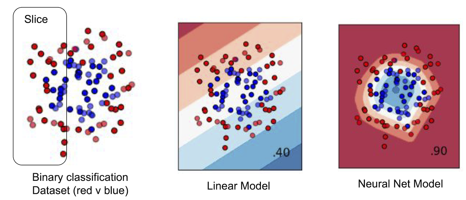 The figure above illustrates an example binary classification task where a linear model must strictly tradeoff between producing worse predictions for data inside the slice vs. outside it. A more flexible neural net model does not have to make this tradeoff and is able to to produce accurate predictions both inside and outside the slice.
 -
Over-sample or up-weight the examples from a minority subgroup that is currently receiving poor predictions. To understand why this might help, consider data from two subgroups which overlap in feature space but tend to have different labels. No model can perform well on such data; a classifier must tradeoff between modeling one class well vs. the other and we can obtain better performance for examples from one subgroup by up-weighting them during training (at the cost of potentially harming performance for other subgroups).
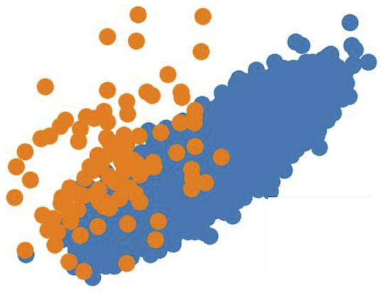 The figure above illustrates an example dataset where the orange and blue subgroups have overlapping feature values. If the labels for these two subgroups tend to differ, then any model will have to tradeoff between producing worse predictions for one subgroup vs. the other. If you assign higher weights to the orange datapoints, then the resulting model should produce better predictions for them at the cost of potentially worse predictions for the blue subgroup.
 -
Collect additional data from the subgroup of interest. To assess whether this is a promising approach: you can re-fit your model to many alternative versions of your dataset in which you have down-subsampled this subgroup to varying degrees, and then extrapolate the resulting model performance that would be expected if you had more data from this subgroup.
-
Measure or engineer additional features that allow your model to perform better for a particular subgroup. Sometimes the provided features in the original dataset may bias results for a particular subgroup. Consider the example of classifying if a customer will purchase some product or not, based on customer & product features. Here predictions for young customers may be worse due to less available historical observations. You could add an extra feature to the dataset specifically tailored to improve predictions for this subgroup such as: “Popularity of this product among young customers”.
Discovering underperforming subpopulations
Some data may not have obvious slices, for example a collection of documents or images. In this case, how can we identify subgroups where our model underperforms?
Here is one general strategy:
- Sort examples in the validation data by their loss value, and look at the examples with high loss for which your model is making the worst predictions (Error Analysis).
- Apply clustering to these examples with high loss to uncover clusters that share common themes amongst these examples.
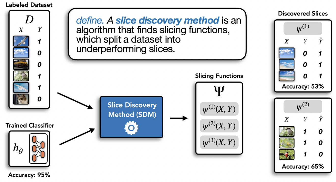
Many clustering techniques only require that you to define a distance metric between two examples [C22]. By inspecting the resulting clusters, you may be able to identify patterns that your model struggles with. Step 2 can also use clustering algorithms that are label or loss-value aware, which is done in the Domino slice discovery method [E22] pictured below.
Why did my model get a particular prediction wrong?
Reasons a classifier might output an erroneous prediction for an example $x$ [S22]:
- The given label is incorrect (and our model actually made the right prediction).
- This example does not belong to any of the $K$ classes (or is fundamentally not predictable, e.g. a blurry image).
- This example is an outlier (there are no similar examples in the training data).
- This type of model is suboptimal for such examples. To diagnose this, you can up-weight this example or duplicate it many times in the dataset, and then and see if the model is still unable to correctly predict it after being retrained. This scenario is hard to resolve via dataset improvement, instead try: fitting different types of models, hyperparameter tuning, and feature engineering.
- The dataset contains other examples with (nearly) identical features that have a different label. In this scenario, there is little you can do to improve model accuracy besides measuring additional features to enrich the data. Calibration techniques may be useful to obtain more useful predicted probabilities from your model.
Recommended actions to construct a better train/test dataset under the first three scenarios above include:
- Correct the labels of incorrectly annotated examples.
- Toss unpredictable examples and those that do not belong to any of the $K$ classes (or consider adding an “Other” class if there are many such examples).
- Toss examples which are outliers in training data if similar examples would never be encountered during deployment. For other outliers, collect additional training data that looks similar if you can. If not, consider a data preprocessing operation that makes outliers’ features more similar to other examples (e.g. quantile normalization of numeric feature, or deleting a feature). You can also use Data Augmentation to encourage your model to be invariant to the difference that makes this outlier stand out from other examples. If these options are infeasible, you can emphasize an outlier in the dataset by up-weighting it or duplicating it multiple times (perhaps with slight variants of its feature values). To catch outliers encountered during deployment, include Out-of-Distribution detection in your ML pipeline [KM22, TMN22].
Quantifying the influence of individual datapoints on a model
As somebody aiming to practice data-centric AI, you may wonder: how would my ML model change if I retrain it after omitting a particular datapoint $(x,y)$ from the dataset?
This question is answered by the influence function $I(x)$. There are many variants of influence that quantify slightly different things, depending on how we define change [J21]. For instance, the change in the model’s predictions vs. the change in its loss (i.e. predictive performance), typically evaluated over held-out data. Here we focus on the latter type of change.
The above is called Leave-one-out (LOO) influence, but another form of influence exists called the Data Shapely value which asks: What is the LOO influence of datapoint $(x,y)$ in any subset of the dataset that contains $(x,y)$? Averaging this quantity over all possible data subsets leads to an influence value that may better reflect the value of $(x,y)$ in broader contexts [J21]. For instance, if there are two identical datapoints in a dataset where omitting both severely harms model accuracy, LOO influence may still conclude that neither is too important (unlike the Data Shapely value).
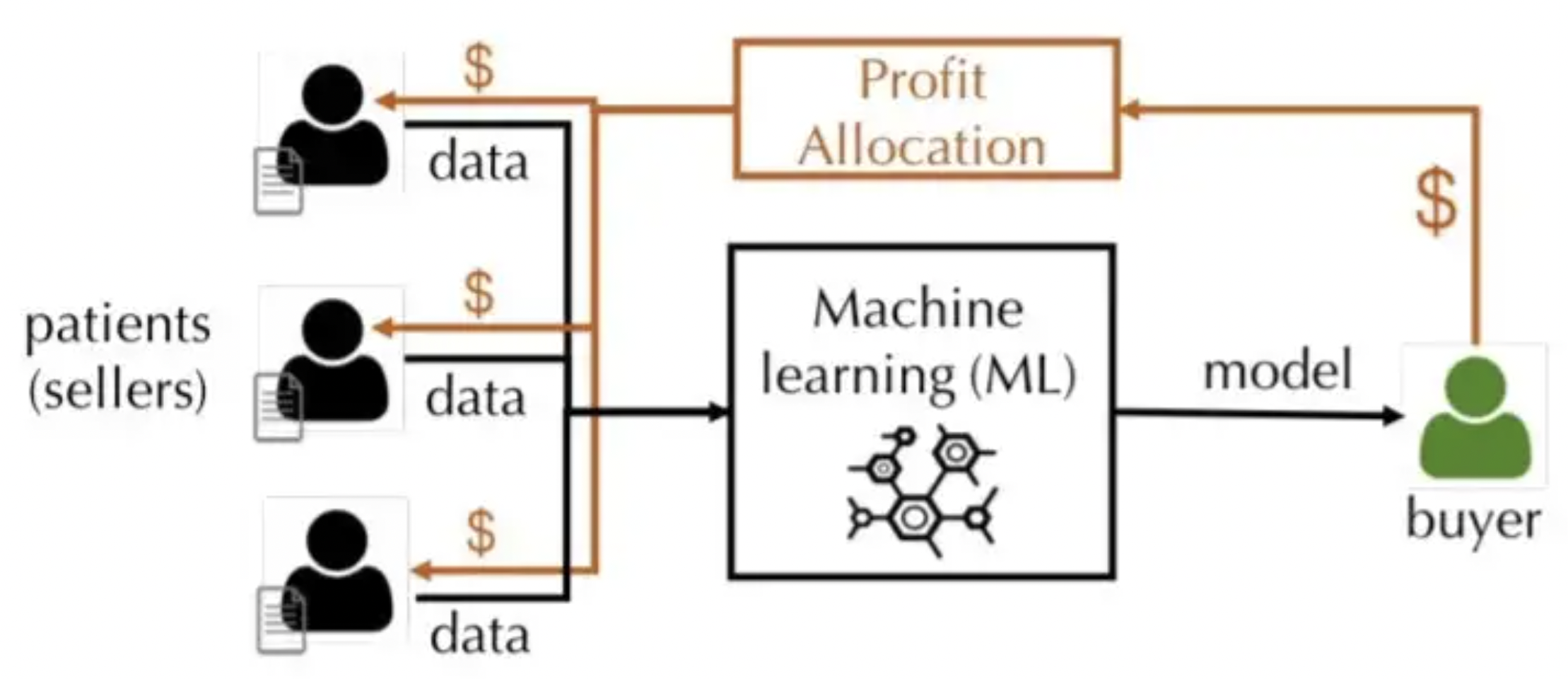
Influence reveals which datapoints have greatest impact on the model. For instance, correcting the label of a mislabeled datapoint with high influence can produce much better model improvement than correcting a mislabeled datapoint that has low influence. $I(x)$ can also be used to assign literal value to data as illustrated in the following figure from [W21]:
Unfortunately, influence can be expensive to compute for an arbitrary ML model. For an arbitrary black-box classifier, you can approximate influence via these Monte-Carlo sampling steps:
- Subsample $T$ different data subsets $\mathcal{D}_t$ from the original training dataset (without replacement).
- Train a separate copy of your model $M_t$ on each subset $\mathcal{D}_t$ and report its accuracy on held-out validation data: $a_t$.
- To assess the value of a datapoint $(x_i,y_i)$, compare the average accuracy of models for those subsets that contained $(x_i,y_i)$ vs. those that did not. More formally:
where $D_\text{in} = \{t : (x_i,y_i) \in \mathcal{D}_t \} $, $ \ D_{\text{out}} = \{t : (x_i,y_i) \notin \mathcal{D}_t \} $.
Accuracy here could be replaced by any other loss of interest.
For special families of models, we can efficiently compute the exact influence function. In a regression setting where we use a linear regression model and the mean squared error loss to evaluate predictions, the fitted parameters of the trained model are a closed form function of the dataset. Thus for linear regresssion, the LOO influence $I(x)$ can be calculated via a simple formula and is also known as Cook’s Distance in this special case [N20].
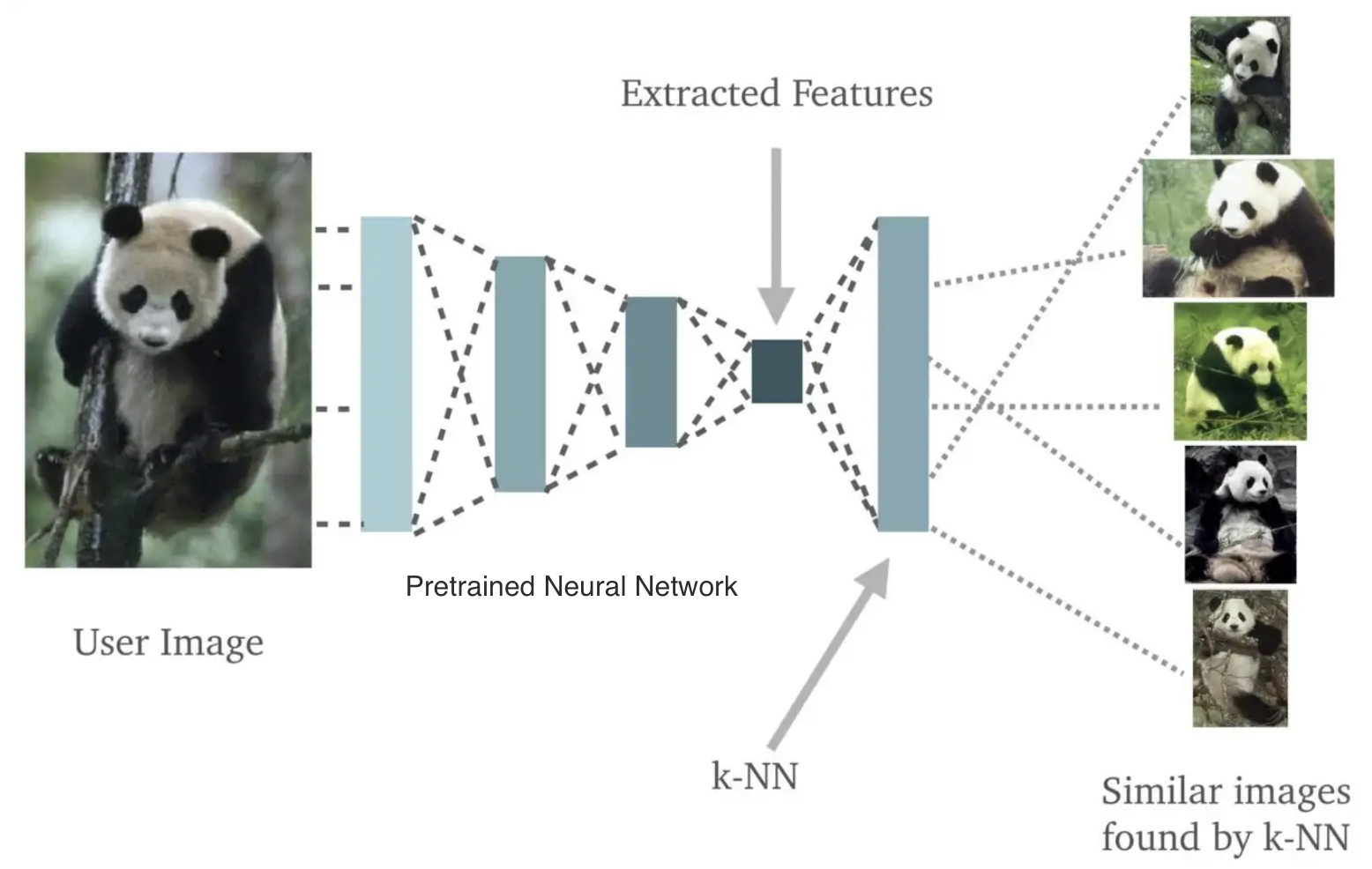
In classification, the influence function can be computed in reasonable $O(n \log n)$ time for a K Nearest Neighbors (KNN) model. For valuation of unstructured data, a general recipe is to use a pretrained neural network to embed all the data, and then apply a KNN classifier on the embeddings, such that the influence of each datapoint can be efficiently computed [J21]. These two steps are illustrated in the following figure from [K18]:
Lab
A hands-on lab assignment to accompany this lecture is available in the dcai-lab repository. The assignment, found in the notebook data_centric_evaluation/Lab – Data-Centric Evaluation.ipynb, is to try improving the performance of a given model solely by improving its training data via some of the various strategies covered here.
References
[R08] Rifkin, R. MIT 9.520 Class Notes on Multiclass Classification. 2008.
[HTF17] Hastie, T., Tibshirani, R. Friedman, J. The Elements of Statistical Learning. 2017.
[Z15] Zheng, A. Evaluating Machine Learning Models. 2015.
[VC22] Varoquaux, G., Colliot, O. Evaluating machine learning models and their diagnostic value. Machine Learning for Brain Disorders, 2022.
[KN22] Kapoor, S., Narayanan, A. Leakage and the Reproducibility Crisis in ML-based Science. 2022.
[O19] Open Data Science. How to Fix Data Leakage — Your Model’s Greatest Enemy. Medium, 2019.
[NAM21] Northcutt, C. G., Athalye, A., Mueller, J. Pervasive Label Errors in Test Sets Destabilize Machine Learning Benchmarks. NeurIPS Track on Datasets and Benchmarks, 2021.
[H18] Hardesty, L. Study finds gender and skin-type bias in commercial artificial-intelligence systems. MIT News, 2018.
[VFK21] Vokinger, K. N., Feuerriegel, S., Kesselheim, A. S., Mitigating bias in machine learning for medicine. Communications Medicine, 2021.
[CJS18] Chen, I. Johansson, F. D., Sontag, D. Why Is My Classifier Discriminatory?. NeurIPS, 2018.
[KGZ19] Kim, M. P., Ghorbani, A., Zou, J. Multiaccuracy: Black-Box Post-Processing for Fairness in Classification. AIES, 2019.
[C22] Clustering. scikit-learn documentation, 2022.
[E22] Eyuboglu et al. Discovering the systematic errors made by machine learning models. ICLR, 2022.
[S22] Sabini, M. Boosting Model Performance Through Error Analysis. Landing.ai Blog, 2022.
[KM22] Kuan, J., Mueller, J. Back to the Basics: Revisiting Out-of-Distribution Detection Baselines. ICML Workshop on Principles of Distribution Shift, 2022.
[TMN22] Tkachenko, U., Mueller, J., Northcutt, C. A Simple Adjustment Improves Out-of-Distribution Detection for Any Classifier. Towards AI, 2022.
[J21] Jia et al. Scalability vs. Utility: Do We Have to Sacrifice One for the Other in Data Importance Quantification? CVPR, 2021.
[W21] Warnes, Z. Efficient Data Valuation with Exact Shapley Values. Towards Data Science, 2021.
[N20] Nguyenova, L. A little closer to Cook’s distance. Medium, 2020.
[K18] Kristiansen, S. Nearest Neighbors with Keras and CoreML. Medium, 2018.
Licensed under CC BY-NC-SA.