Data-Centric AI vs. Model-Centric AI

Click here to view the raw lecture video on Panopto.
An edited version of this video will be posted after the course is over.

Slides: [pdf, pptx]

When you learn Machine Learning in school, a dataset is given to you that is fairly clean & well-curated (e.g. dog/cat images), and your job is to produce the best model for this dataset. All techniques taught in most ML classes are centered around this aim, covering different types of: models (neural networks, decision trees, etc.), training techniques (regularization, optimizaton algorithms, loss functions, etc.), and model/hyperparameter selection (plus model ensembling). We call this paradigm model-centric AI.

When working on real-world ML, your company/users do not care what clever modeling tricks you know to produce accurate predictions on highly curated data. Contrary to the classroom, the data are not fixed in real-world applications! You are free to modify the dataset in order to get better modeling performance or even collect additional data as your budget allows. Real-world data tends to be highly messy and plagued with issues, such that improving the dataset is a prerequisite for producing an accurate model (“garbage in, garbage out”). Seasoned data scientists know it is more worthwhile to invest in exploring and fixing the data than tinkering with models, but this process can be cumbersome for large datasets. Improving data has been mostly done in an ad hoc manner via manual labor guided by human intuition/expertise.

In this class, you will instead learn how to systematically engineer data to build better AI systems. We call this paradigm data-centric AI [G21]. While manual exploratory data analysis is a key first step of understanding and improving any dataset, data-centric AI uses AI methods to more systematically diagnose and fix issues that commonly plague real-world datasets. Data-centric AI can take one of two forms:

1. AI algorithms that understand data and use that information to improve models. Curriculum learning is an example of this, in which ML models are trained on ‘easy data’ first [B09].

2. AI algorithms that modify data to improve AI models. Confident learning is an example of this, in which ML models are trained on a filtered dataset where mislabeled data has been removed [NJC21].

In both examples above, determining which data is easy or mislabeled is estimated automatically via algorithms applied to the outputs of trained ML models.

A practical recipe for supervised Machine Learning

To recap: model-centric AI is based on the goal of producing the best model for a given dataset, whereas data-centric AI is based on the goal of systematically & algorithmically producing the best dataset to feed a given ML model. To deploy the best supervised learning systems in practice, one should do both. A data-centric AI pipeline can look like this:

1. Explore the data, fix fundamental issues, and transform it to be ML appropriate.

2. Train a baseline ML model on the properly formatted dataset.

3. Utilize this model to help you improve the dataset (techniques taught in this class).

4. Try different modeling techniques to improve the model on the improved dataset and obtain the best model.

Remember not to skip straight from Step 2 to Step 4 even though it is tempting! To deploy the best ML systems, one can iterate Steps 3 and 4 multiple times.

Examples of data-centric AI

Methodologies that fall within the purview of this field include:

• Outlier detection and removal (handling abnormal examples in dataset)
• Error detection and correction (handling incorrect values/labels in dataset)
• Establishing consensus (determining truth from many crowdsourced annotations)
• Data augmentation (adding examples to data to encode prior knowledge)
• Feature engineering and selection (manipulating how data are represented)
• Active learning (selecting the most informative data to label next)
• Curriculum learning (ordering the examples in dataset from easiest to hardest)

Recent high-profile ML applications have clearly shown how the reliability of ML models deployed in the real-world depends on the quality of their training data.

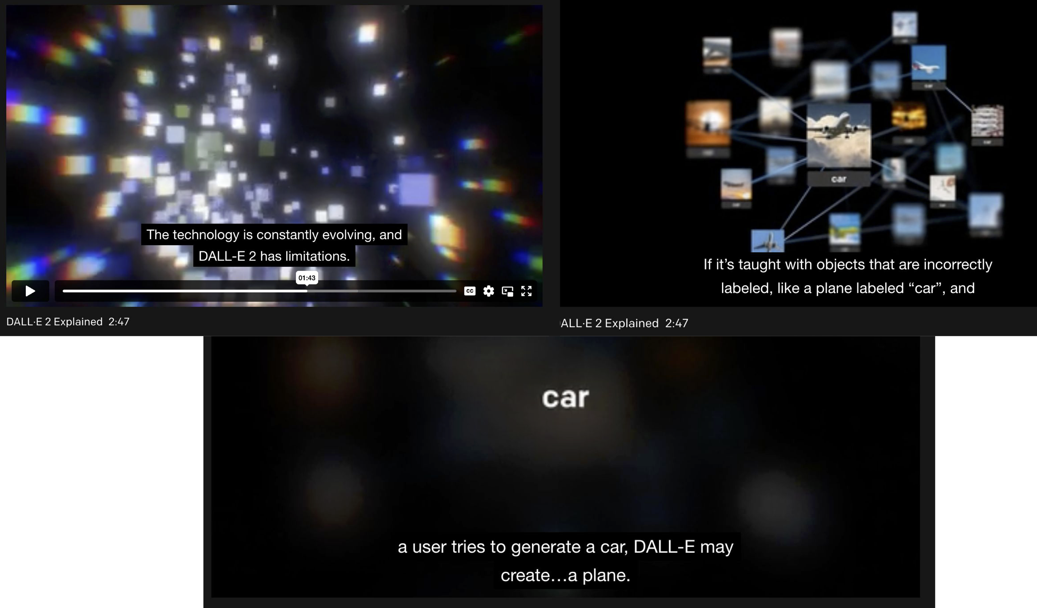
OpenAI has openly stated that one of the biggest issues in training famous ML models like Dall-E, GPT-3, and ChatGPT were errors in the data and labels. Here are some stills from their video demo of Dall-E 2:

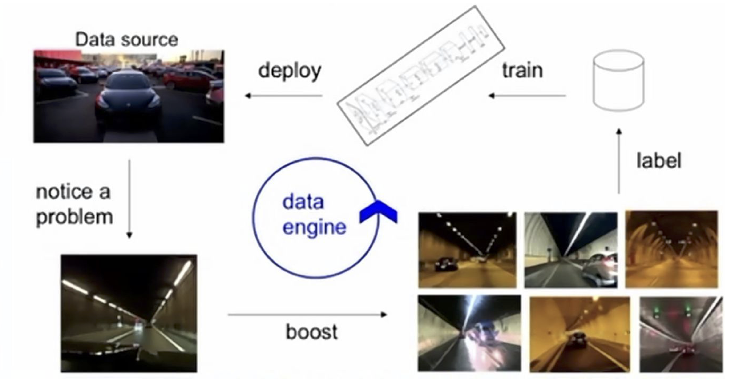
Through relentless model-assisted dataset improvement (Step 3 above), Tesla could produce autonomous driving systems far more advanced than similar competitors. They point to their Data Engine as the key reason from this success, depicted in the following slides from Andrej Karpathy, the Tesla Director of AI (2021):

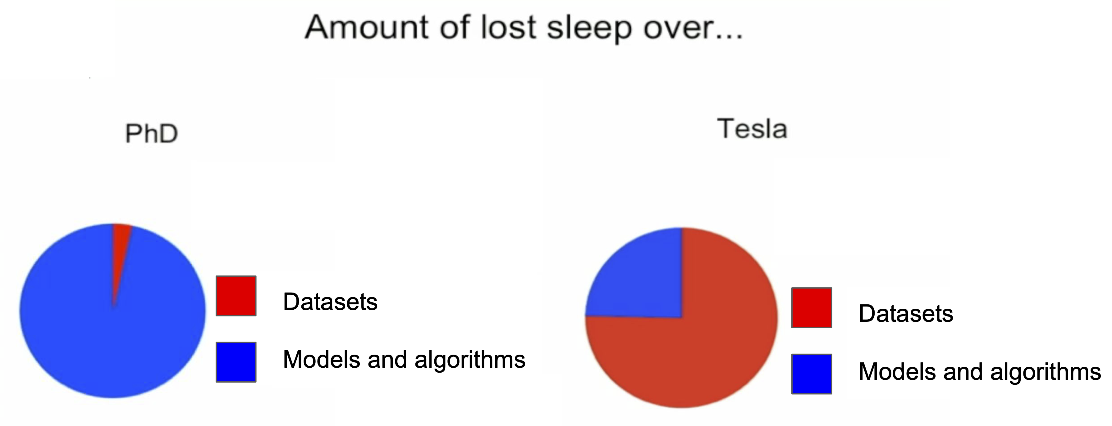
Why we need data-centric AI

Bad data costs the U.S. alone around $3 Trillion every year [R16]. Data quality issues plague almost every industry and dealing with them manually imposes an immense burden. As datasets grow larger, it becomes infeasible to ensure their quality without the use of algorithms [S22]. Recent ML systems trained on massive datasets like ChatGPT have relied on huge amounts of labor (human feedback) to try to overcome shortcomings arising from low-quality training data; however such efforts have been unable to fully overcome these shortcomings [C23]. Now more than ever, we need automated methods and systematic engineering principles to ensure ML models are being trained with clean data. As ML becomes intertwined with our daily lives in healthcare, finance, transportation, it is imperative these systems are trained in a reliable manner.

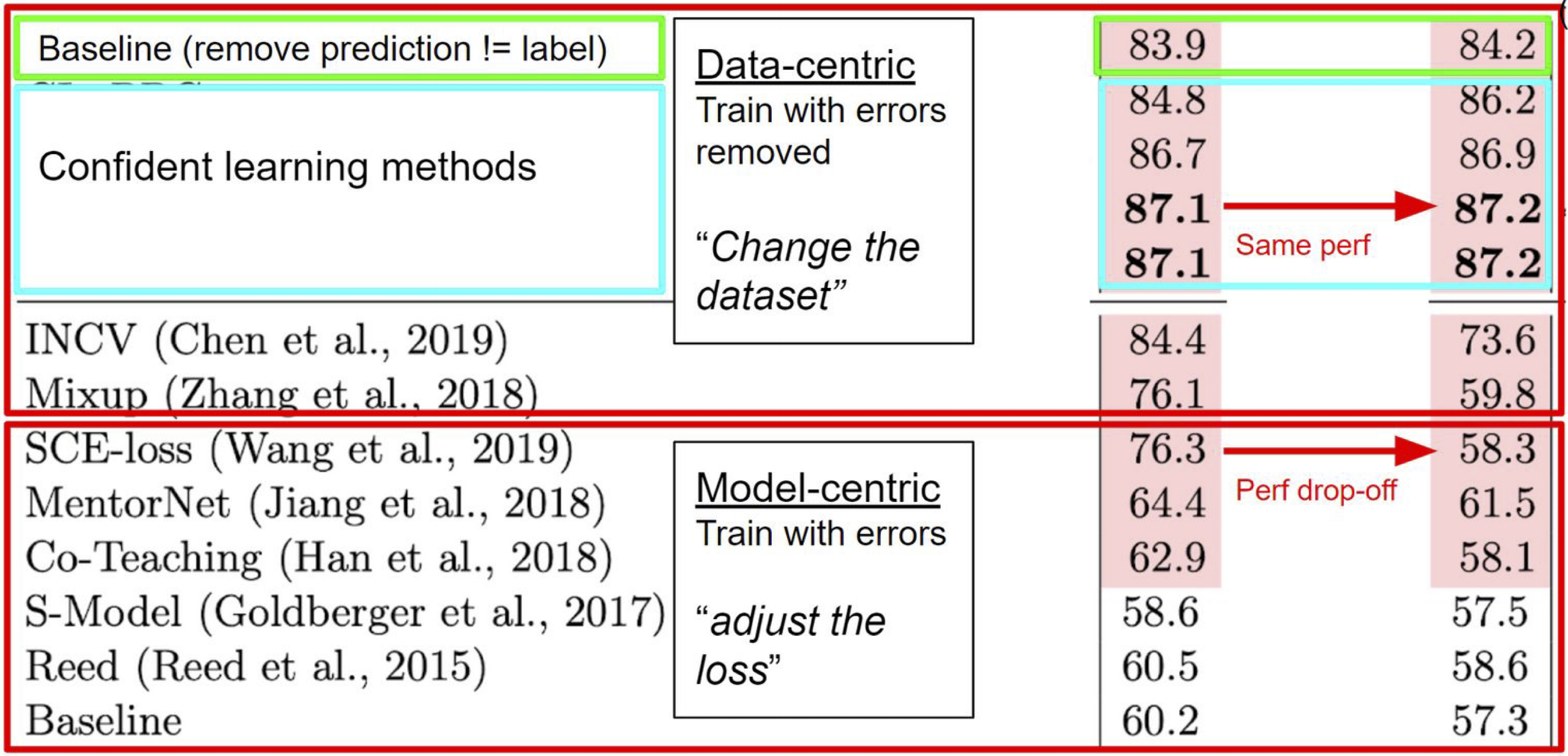
Recent research is highlighting the value of data-centric AI for various applications. For image classification with noisily labeled data, a recent benchmark studied various methods to train models under increasing noise rates in the famous Cifar-10 dataset [NJC21]. The findings revealed that simple methods which adaptively change the dataset can lead to much more accurate models than methods which aim to account for the noise through sophisticated modeling strategies.

Now that you’ve seen the importance of data-centric AI, this class will teach you techniques to improve any ML model by improving its data. The techniques taught here are applicable to most supervised ML models and training techniques, such that you will be able to continue applying them in the future even as better ML models and training techniques are invented. The better models of the future will better help you find and fix issues in datasets when combined with the techniques from this course, in order to help you produce even better versions of them!

The perceptron of data-centric AI: PU learning

The perceptron of machine learning

In many machine learning courses, in the first lecture you learn about the perceptron algorithm, a simplified version of SGD that produces a linear classifier for the binary classification task of predicting whether an example $x_i$ has a label $y_i$ belonging to class $0$ or class $1$.

Our goal: estimate the binary classifier $f(x) = p(y = 1 \mid x)$ from data $(x_i, y_i): x \in \mathcal{R}^d, y \in {0, 1}, i \in {1 \ldots n}$

The algorithm: the perceptron algorithm is an iterative algorithm (time-step $t$) that trains $f(x, t)$ repeatedly on the entire dataset $x_i, y_i : i \in {1 \ldots n}$

For weights $z: 0 \ldots d$ and training example $(x_i, y_i)$ and learning rate $0 \leq \eta \leq 1$, the predicted label $\hat{y}_i(t)$ for $x_i$ is:

where the training algorithm to compute $w(t)$ is iteratively computed

where the term $(y_i - \hat{y}_i(t)) x_{i, z}$ is often referred to as the objective function and the negative of this $-((y_i - \hat{y}_i(t)) \cdot x_{i, z})$ is referred to as the loss function.

We learn the preceptron algorithm at the start of machine learning courses and books because it is a great way to introduce folks to deep learning, since that training algorithm above is very similar to the training algorithm for neural networks and deep learning, called Stochastic Gradient Descent, or for short, SGD:

where $L$ is the loss function of a neural network and $n$ is the total number of examples in your training dataset. The rest of the variables are essentially the same as in the perceptron training step.

If you are unfamiliar with SGD and perceptron, the rest of this course will likely be too challenging and you are encouraged to pick up an ML book and start reading (e.g. Christopher Bishop’s Pattern Recognition and Machine Learning book).

PU learning: The “perceptron” of DCAI

One of the easiest ways to get our feet wet with DCAI is with Positive-Unlabeled (PU) Learning [EN08], one of the first algorithms for systematically improving a binary classifier trained on noisy labels.

Positive-unlabeled (PU) learning is a binary classification task in which a subset of positive training examples is labeled, and the rest are unlabeled. In practice, we assume the positive class is class $1$ and the unlabeled class is class $0$ where some of the labels are noisy (the underlying true label might be $1$ but we just assume everything that is unlabeled is class $0$ when we train our classifier on the training data).

Notationally, for PU learning, each datapoint is a triplet of random variables $(x_i, \tilde{y}_i, y^*_i)$, where

• $x_i \in \mathcal{R}^d$ is the $i^{th}$ example (an image embedding, a text embedding, tabular data, etc) in a dataset of $n$ examples,

• $\tilde{y}_i$ is the noisy observed label associated with example $x_i$, and

• $y^*_i$ is the (unobserved, not known!) latent true label of example $x_i$.

Our goal: is the same as standard binary classification: estimate the binary classifier $f(x) = p(y^* = 1 \mid x)$ from data $(x_i, y^*_i): x \in \mathcal{R}^d, y^* \in {0, 1}, i \in {1 \ldots n}$. Unfortunately, we do not have the true labels $y^*$, we only observe the noisy, erroneous labels $\tilde{y}$. Thus, instead when we train on our observed data $(x_i, \tilde{y}_i) \in {1 \ldots n}$, we estimate the erroneous binary classifier $\tilde{f}(x) = p(\tilde{y} = 1 \mid x)$ instead!

Intermediate goal: Estimate $f(x) = p(y^* = 1 \mid x)$ from $\tilde{f}(x) = p(\tilde{y} = 1 \mid x)$ without observing $y^*$.

The above should seem somewhat magical to you without any assumptions. We estimate the true classifier as if it were trained on perfect labels, even though the labels that are given to us contain wrong labels!

Key Idea: $p(y^* = 1 \mid x) \; = \; p(\tilde{y} = 1 \mid x) \cdot p(\tilde{y} = 1 \mid x, y^* = 1)$

Assumptions: PU learning has a couple of major simplifying assumption that makes it easy to get closed form solutions and makes it a great place to get started learning about the algorithms behind Data-centric AI and data curation.

Assumption 1 (no error in positive labels): PU learning* assumes perfect (error-free) positive labels. Formally, \(p(\tilde{y}=1 \mid x, y^*=0) = 0\)

Assumption 2 (Conditional Independence): PU learning assumes that the probability of the label being flipped from $1$ to $0$ in the unlabeled ($0$ class) does not depend on the data itself.

Formally:

which we can also express in the following way:

because $p(\tilde{y} = 1 \mid y^* = 1) + p(\tilde{y} = 0 \mid y^* = 1) = 1$

and similarly $p(\tilde{y} = 1 \mid x, y^* = 1) + p(\tilde{y} = 0 \mid x, y^* = 1) = 1$.

Key insight

Lemma 1: Suppose the “conditional independence” assumption holds. Then $p(y^* = 1 \mid x) = \frac{p(\tilde{y} = 1 \mid x)}{c}$ where $c = p(\tilde{y} = 1 \mid y^* = 1)$.

Proof: Remember that the assumption is $p(\tilde{y} = 1 \mid y^* = 1, x) = p(\tilde{y} = 1 \mid y^* = 1)$. Now consider $p(\tilde{y} = 1 \mid x)$. We have that

Basics of the PU Learning Algorithm: This is a constructive proof: by computing $c = p(\tilde{y} = 1 \mid y^* = 1)$, you can estimate the more accurate binary classifier you want $f(x) = p(y^* = 1 \mid x)$ from the noisy binary classifier you end up with $\tilde{f}(x) = p(\tilde{y} = 1 \mid x)$ from training on erroneous labels.

Estimating $c = p(\tilde{y} = 1 \mid y^* = 1)$

To obtain $f(x) = p(y^* = 1 \mid x)$ from $\tilde{f}(x) = p(\tilde{y} = 1 \mid x)$ requires a single constant factor $c = p(\tilde{y} = 1 \mid y^* = 1)$. There are multiples ways to estimate $c$. One way (that’s simple, performs well, and is one line of code to implement), is as follows:

where $\tilde{c}$ is an estimator of the true $c$ and $\mathcal{P}$ is the set of positively labeled data (which by definition does not have errors in PU learning).

The intuition for the above is: $\hat{p}(\tilde{y} = 1 \mid x \in \mathcal{P}) \to \hat{p}(\tilde{y} = 1 \mid y^* = 1)$ in the limit as $\vert \mathcal{P} \vert \to \infty$. Keep in mind that $\hat{p}$ is the output of a model and is just an estimate of $p$ so the resulting $\tilde{c}$ is just an estimate averaged over the error in the predicted probabilities of the model.

We can verify this formally as follows:

Show that:

Proof:

Putting it all together: PU Learning Algorithm

To implement PU learning on a computer yourself, the steps are as follows:

Train step

Obtain out-of-sample predicted probabilities from your binary classifier by training on your dataset out of sample (you can do this using cross-validation… i.e., train on all of the data except a slice, then predict on that slice, then repeat for all slices, then np.concat the predicted probabilities back together.

Now you should have $\hat{p}(\tilde{y} = 1 \mid x)$ for all your training data. It is important to train out of sample otherwise the predicted probabilities will overfit to 0 and 1 since the classifier has already seen the data.

Characterize error (DCAI) step

Compute $\tilde{c} = \frac{1}{\mid \mathcal{P} \mid} \sum_{x \in \mathcal{P}} \hat{p}(\tilde{y} = 1 \mid x)$

Final training step

Toss out all previous predicted probabilities and classifiers. Starting from scratch, train a new classifier on your entire dataset (no need to do cross-validation here; just train on all the data at once). The point here is to get a classifier trained on 100% of your data to maximize performance. Let us call this trained model $\tilde{f}$.

Inference step

$f(x_{\text{new}}) = p(y^* = 1 \mid x_{\text{new}}) = \frac{p(\tilde{y} = 1 \mid x_{\text{new}})}{c}$.

The classification of new data is the rule: if $f(x_{\text{new}}) >= 0.5$ then predict $x_{\text{new}}$ is class 1 else predict $x_{\text{new}}$ is class 0 .

Next up: Confident Learning

The PU learning approach introduced by [EN08] is an insightful first leap into the world of systematic model improvement on imperfect data. But this approach isn’t without its caveats. It is a highly restricted case (one of the classes must be perfect and it only works for binary classification).

This method is also sensitive to the accuracy of the model’s predicted probabilities since $c = p(\tilde{y} = 1 \mid y^* = 1)$ is calculated by averaging predicted probabilities.

Next lecture, we will unveil how you can estimate $f(x)$ without these assumptions for the general case (multi-class classification – applicable to most real-world datasets (e.g. language models, computer vision models, etc.). This is an area of machine learning that automatically finds label errors in any multi-class ML dataset known as “confident learning” developed here at MIT [NJC21]. Confident learning introduces robustness to imperfect model predicted probabilities, generalized to any number of classes, and allow any class to be mislabeled as any other class.

Lab

Lab assignments for each lecture in this course are available in the dcai-lab GitHub repository. Get started with:

$ git clone https://github.com/dcai-course/dcai-lab

Remember to run a git pull before doing every lab, to make sure you have the latest version of the labs. Alternatively you can just download individual files yourself from dcai-lab.

The first lab assignment, in data_centric_model_centric/Lab - Data-Centric AI vs Model-Centric AI.ipynb, walks you through an ML task of building a text classifier, and illustrates the power (and often simplicity) of data-centric approaches.

References

[EN08] Elkan, C. and Noto, K. Learning Classifiers from Only Positive and Unlabeled Data. KDD, 2008.

[G21] Press, G. Andrew Ng Launches A Campaign For Data-Centric AI. Forbes, 2021.

[B09] Bengio, Y., et al. Curriculum Learning. ICML, 2009.

[NJC21] Northcutt, C., Jiang, L., Chuang, I.L. Confident Learning: Estimating Uncertainty in Dataset Labels. Journal of Artifical Intelligence Research, 2021.

[R16] Redman, T. Bad Data Costs the U.S. $3 Trillion Per Year. Harvard Business Review, 2016.

[S22] Strickland, E. Andrew Ng: Unbiggen AI. IEEE Spectrum, 2022.

[C23] Chiang, T. ChatGPT is a Blurry JPEG of the Web. New Yorker, 2023.